Starfile

import os

import matplotlib.pyplot as plt
import numpy as np

from aspire.noise import AnisotropicNoiseEstimator
from aspire.reconstruction import MeanEstimator
from aspire.source import RelionSource

Sources

Sources are an interface to various backend stores of data (np arrays, starfiles, etc) They are intended to handle batching data conversion/prep behind the scenes. Here we load a “.star” file using the RelionSource class

data_folder = os.path.join(os.path.dirname(os.getcwd()), "data")
file_path = os.path.join(data_folder, "sample_relion_data.star")

source = RelionSource(
    file_path,
    pixel_size=1.338,
    max_rows=10000,
    data_folder=data_folder,
)

# Reduce the resolution
L = 12  # You may try 16 but it takes a significant amount of time.
source = source.downsample(L)

Noise Estimation and Whitening

# Estimate noise in the ImageSource instance
noise_estimator = AnisotropicNoiseEstimator(source)
# Apply whitening to ImageSource
source = source.whiten(noise_estimator)

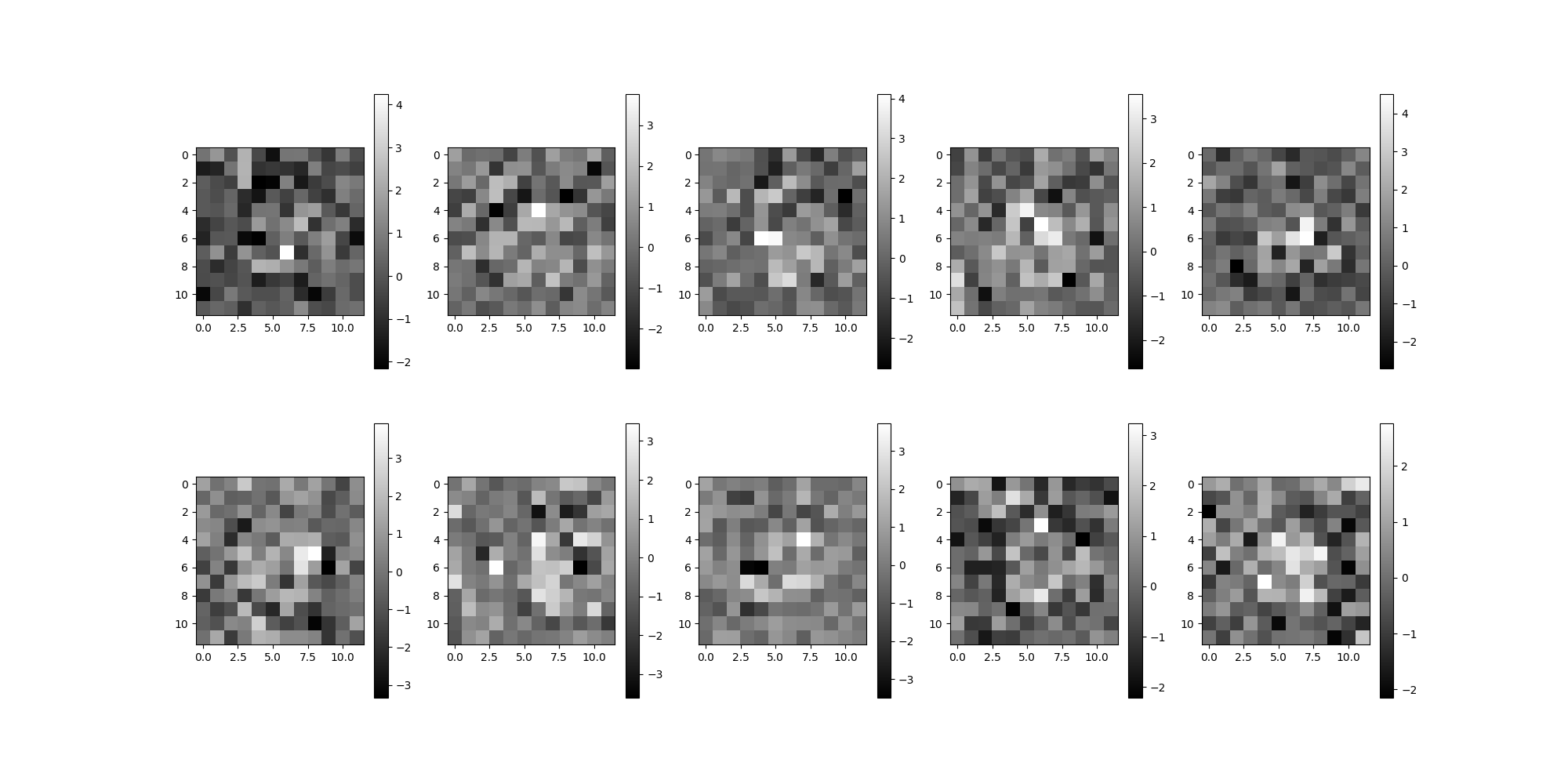
# Display subset of the images
images = source.images[:10]
images.show()

  0%|          | 0/1 [00:00<?, ?it/s]
100%|██████████| 1/1 [00:00<00:00, 103.61it/s]

Estimate Mean Volume

# Estimate mean Volume
mean_estimator = MeanEstimator(source, batch_size=8192)
mean_est = mean_estimator.estimate()

Visualize Volume

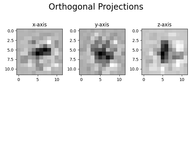
# MeanEstimator.estimate() returns a Volume Instance,
#   which is wrapper on an ndarray representing a stack of one or more 3d volumes.
# We will visualize the data via orthogonal projections along the three axes.

vol = mean_est.asnumpy()[0]
# Visualize volume
L = vol.shape[0]
# Plots
plt.suptitle("Orthogonal Projections", size=20)
plt.subplot(1, 3, 1, title="x-axis")
plt.imshow(np.sum(vol, axis=0), cmap="gray")
plt.subplot(1, 3, 2, title="y-axis")
plt.imshow(np.sum(vol, axis=1), cmap="gray")
plt.subplot(1, 3, 3, title="z-axis")
plt.imshow(np.sum(vol, axis=2), cmap="gray")
plt.tight_layout()
plt.subplots_adjust(top=1.25)
plt.show()