Micrograph Sources

This tutorial will demonstrate how to set up and use ASPIRE’s MicrographSource classes.

import os
import tempfile

import numpy as np

from aspire.source import ArrayMicrographSource

Overview

MicrographSource is an abstract class which provides access to three distinct subclasses. The first two are ArrayMicrographSource and DiskMicrographSource which provide access to array and disk backed micrograph data respectively. MicrographSimulation takes a volume and generates projection images which are aggregated into synthetic microgaphs. The following illustrates an overview of the interfaces, and the tutorial will go on to demonstrate common operations for each class.

classDiagram class MicrographSource{ micrograph_count: int micrograph_size: int dtype: np.dtype +asnumpy() +dtype +len() +repr() +images[] +micrograph_count +micrograph_size +save() +show() } class ArrayMicrographSource{ micrographs: np.ndarray } class DiskMicrographSource{ micrographs_path: str, Path, or list } class MicrographSimulation{ volume: Volume micrograph_size: Optional, int micrograph_count: Optional, int particles_per_micrograph: Optional, int particle_amplitudes: Optional, np.ndarray projection_angles: Optional, np.ndarray seed: Optional, int ctf_filters: Optional, list noise_adder: Optional, NoiseAdder boundary: Optional, int interparticle_distance: Optional, int +boundary +centers +ctf_filters +clean_images[] +filter_indices +get_micrograph_index() +get_particle_index() +interparticle_distance +noise_adder +simulation +particle_amplitudes +particle_box_size +particle_per_micrograph +projection_angles +total_particle_count +volume } MicrographSource <|-- ArrayMicrographSource MicrographSource <|-- DiskMicrographSource MicrographSource <|-- MicrographSimulation MicrographSimulation o-- Volume MicrographSimulation *-- CTFFilter MicrographSimulation *-- NoiseAdder

Creating an ArrayMicrographSource

An ArrayMicrographSource is populated with an array. For this demonstration, random data will initialize the object, then this data will be saved off for use in the next example (which loads data from files).

# Create an (2,512,512) array of data.
# This represents two (512,512) micrographs.
mgs_np = np.random.rand(2, 512, 512)

# Construct the source
src = ArrayMicrographSource(mgs_np)

# Create a tmp dir for saving the data to.
# This just for ensuring the tutorial script is portable,
tmp_dir = tempfile.TemporaryDirectory()

# Save the data as multiple MRC files
# This method returns a file_list,
# which might be useful for loading or other operations.
file_list = src.save(tmp_dir.name)

Creating a DiskMicrographSource

A DiskMicrographSource is populated with str or list representing the location of MRC files.

from aspire.source import DiskMicrographSource

# Load files in directory
src = DiskMicrographSource(tmp_dir.name)

# Load files from a list
src = DiskMicrographSource(file_list)

Creating a Micrograph Simulation

A MicrographSimulation is populated with particle projections from a Volume, so we’ll begin by generating a Volume.

from aspire.source import MicrographSimulation
from aspire.volume import AsymmetricVolume

# Generate one (100,100,100) ``Volume``.
vol = AsymmetricVolume(
    L=100,
    C=1,
    seed=1234,
    dtype=np.float32,
).generate()

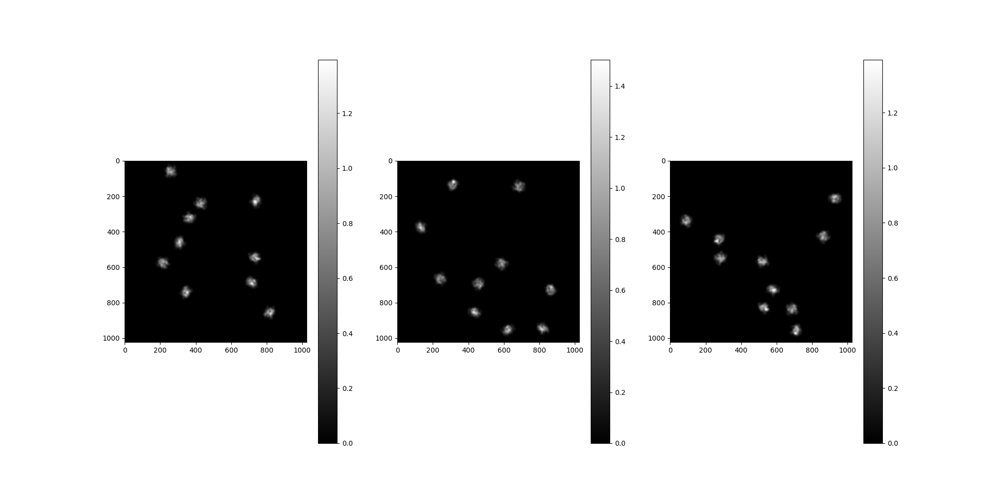
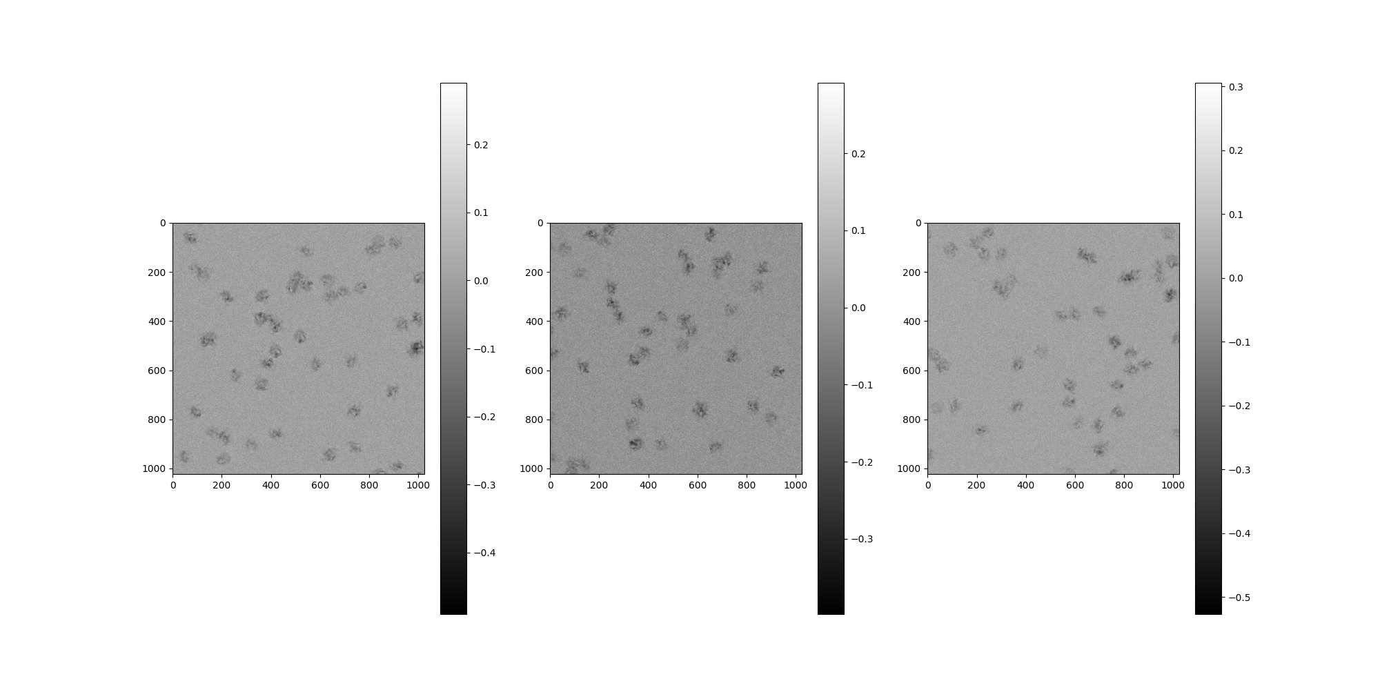
We’ll pass our Volume as an argument and configure our MicrographSimulation. In this example, the MicrographSimulation has 4 micrographs of size 1024, each with 10 particles.

n_particles_per_micrograph = 10
n_micrographs = 3

src = MicrographSimulation(
    vol,
    particles_per_micrograph=n_particles_per_micrograph,
    particle_amplitudes=1,
    micrograph_size=1024,
    micrograph_count=n_micrographs,
    seed=1234,
)

# Plot the micrographs
src.images[:].show()

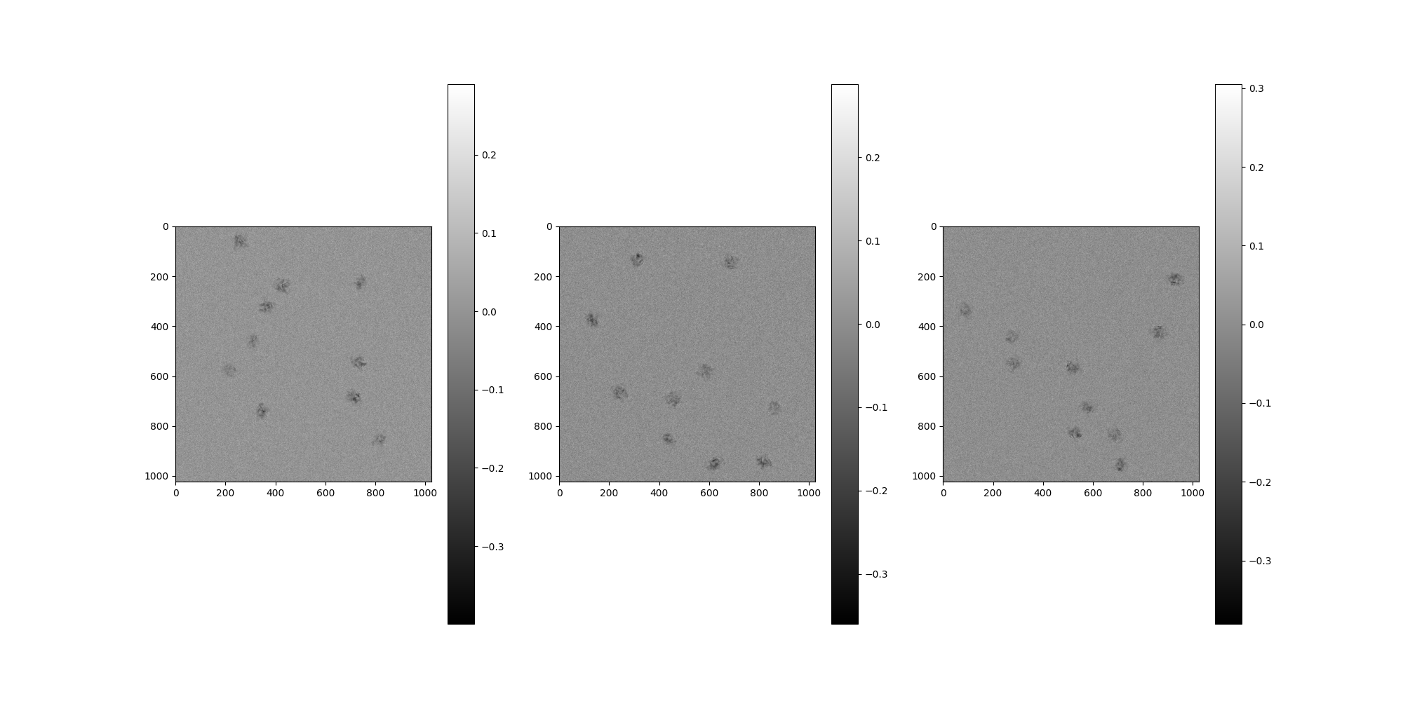
CTF Filters

By default, no CTF corruption is configured. To apply CTF filters, we have to pass them as arguments to the MicrographSimulation. It is possible to apply a single CTF, different CTF per-micrograph or different CTF per-particle by configuring a list of matching size.

from aspire.operators import RadialCTFFilter

# Create our CTF Filter and add it to a list.
# This configuration will apply the same CTF to all particles.
ctfs = [
    RadialCTFFilter(pixel_size=4, voltage=200, defocus=15000, Cs=2.26, alpha=0.07, B=0),
]

src = MicrographSimulation(
    vol,
    particles_per_micrograph=n_particles_per_micrograph,
    micrograph_size=1024,
    micrograph_count=n_micrographs,
    ctf_filters=ctfs,
    seed=1234,
)

# Plot the micrographs
src.images[:].show()

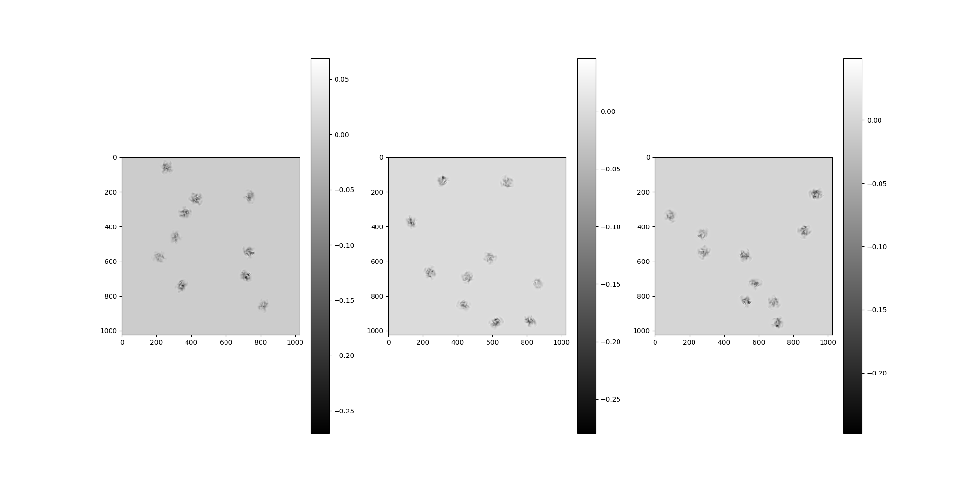
Noise

By default, no noise corruption is configured. To apply noise, pass a NoiseAdder to MicrographSimulation.

from aspire.noise import WhiteNoiseAdder

# Create our noise using WhiteNoiseAdder
noise = WhiteNoiseAdder(4e-3, seed=1234)

# Add noise to our MicrographSimulation using the noise_adder argument
src = MicrographSimulation(
    vol,
    noise_adder=noise,
    particles_per_micrograph=n_particles_per_micrograph,
    micrograph_size=1024,
    micrograph_count=n_micrographs,
    ctf_filters=ctfs,
    seed=1234,
)

# Plot the micrographs
src.images[:].show()

Plot the clean micrographs using the clean_images accessor.

src.clean_images[:].show()

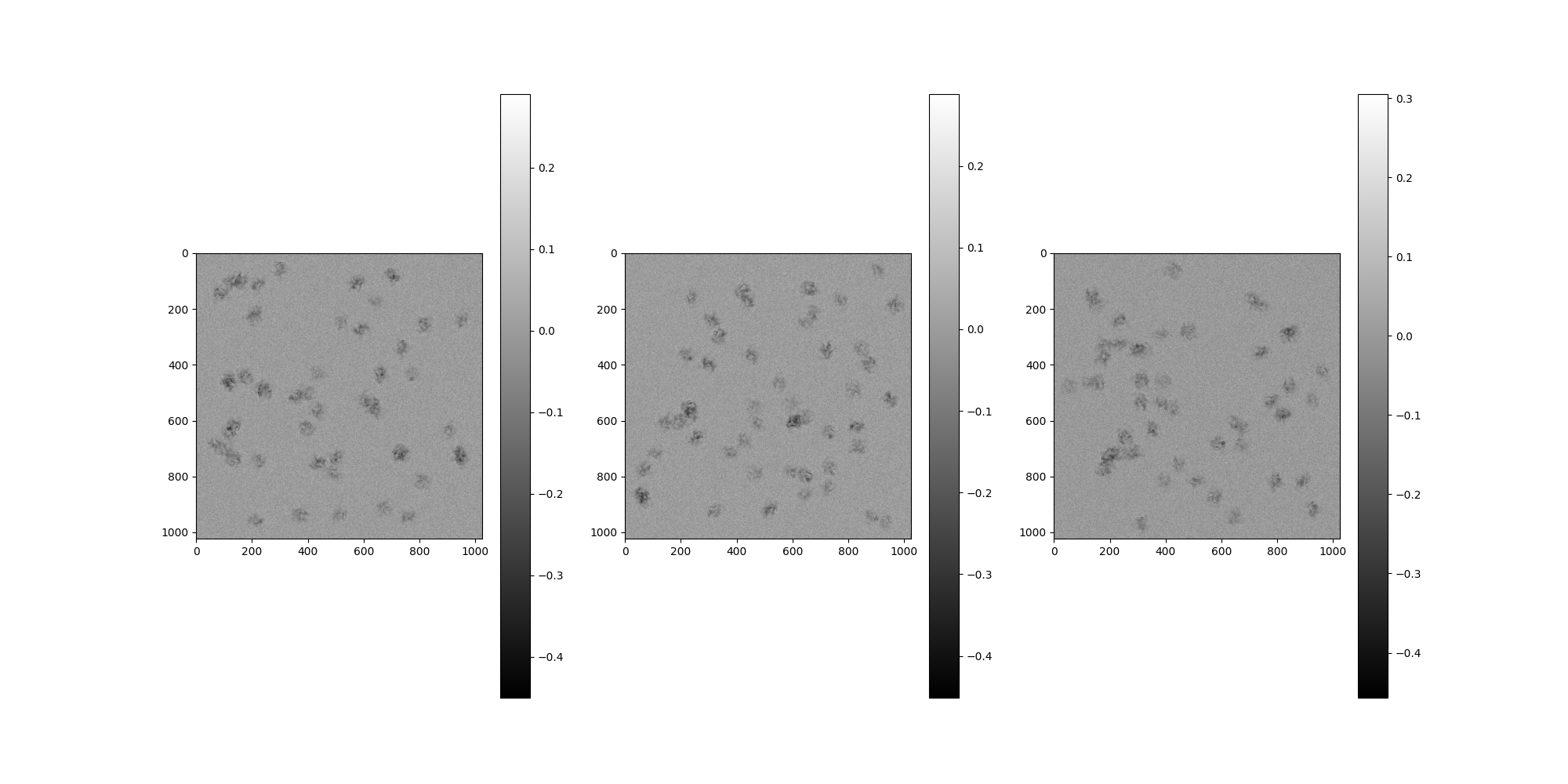
Interparticle Distance

By default, particle distance is set to avoid collisions. We can use the interparticle_distance argument to control the minimum distance between particle centers. However, setting this argument too large may generate insufficient centers.

# Let's increase the number of particles to show overlap.
n_particles_per_micrograph = 50

# Set the interparticle distance to 1, which adds at least one pixel
# of separation between center and allows particles to collide.
src = MicrographSimulation(
    vol,
    interparticle_distance=1,
    noise_adder=noise,
    particles_per_micrograph=n_particles_per_micrograph,
    micrograph_size=1024,
    micrograph_count=n_micrographs,
    ctf_filters=ctfs,
)

# Plot the micrographs
src.images[:].show()

Boundary

By default, the boundary is set to half of the particle width, which will completely contain every particle inside the micrograph. Setting boundary=0 will allow particles to be placed along the edges. Positive values (measured in pixels) move the boundaries inward, while negative values move the boundaries outward.

# Create a micrograph with a negative boundary, allowing particles to
# generate outward.
out_src = MicrographSimulation(
    vol,
    boundary=-20,
    interparticle_distance=1,
    noise_adder=noise,
    particles_per_micrograph=n_particles_per_micrograph,
    micrograph_size=1024,
    micrograph_count=n_micrographs,
    ctf_filters=ctfs,
)

# Plot the micrographs
out_src.images[:].show()

Particle Indices

Each particle comes from a Simulation internal to MicrographSimulation. This simulation can be accessed directly by the attribute MicrographSimulation.simulation. A map is provided between each particle’s indexing relative to that Simulation and micrograph based indexing. This relationship is demonstrated below.

# Let's choose four random numbers as our global (``Simulation``)
# particle indices from ``test_micrograph=1``.
test_micrograph = 1
n_particles = 3
local_particle_indices = np.random.choice(n_particles_per_micrograph, n_particles)
print(f"Local particle indices: {local_particle_indices}")

Local particle indices: [24 20 36]

We can obtain the individual particle images from our MicrographSimulation by retrieving their centers and plotting the boundary boxes.

centers = np.zeros((n_particles, 2), dtype=int)
for i in range(n_particles):
    centers[i] = src.centers[test_micrograph][local_particle_indices[i]]

# Let's use the particles' centers and sizes to perform "perfect
# particle picking" on this test micrograph.
p_size = src.particle_box_size
micrograph_picked_particles = np.zeros(
    (
        n_particles,
        src.particle_box_size,
        src.particle_box_size,
    )
)

for i, center in enumerate(centers):
    x, y = center[0], center[1]
    # Calculate the square of the particle
    particle = src.clean_images[test_micrograph].asnumpy()[0][
        x - p_size // 2 : x + p_size // 2, y - p_size // 2 : y + p_size // 2
    ]
    micrograph_picked_particles[i] = particle

# Let's plot and look at the particles!
from aspire.image import Image

Image(micrograph_picked_particles)[:].show()

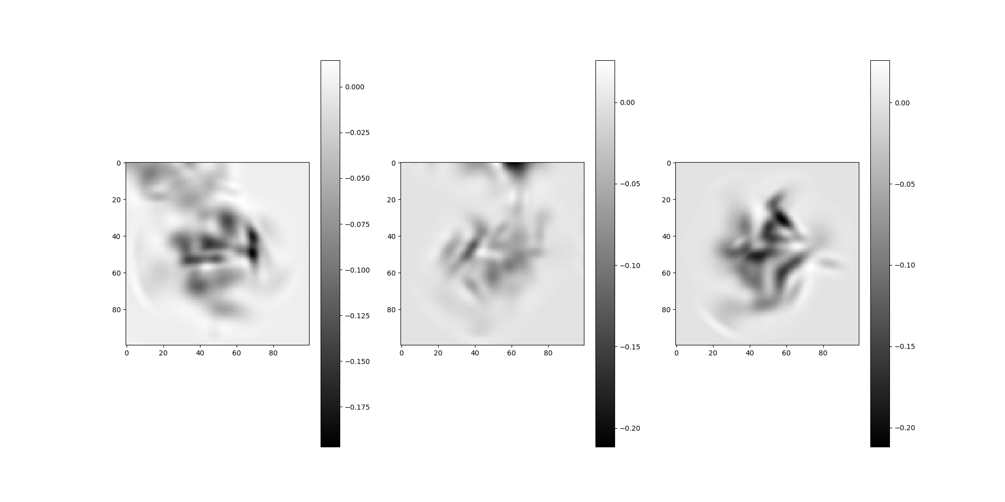
Note

There may be overlap with nearby particles in the above images. To reduce overlap, increase interparticle_distance.

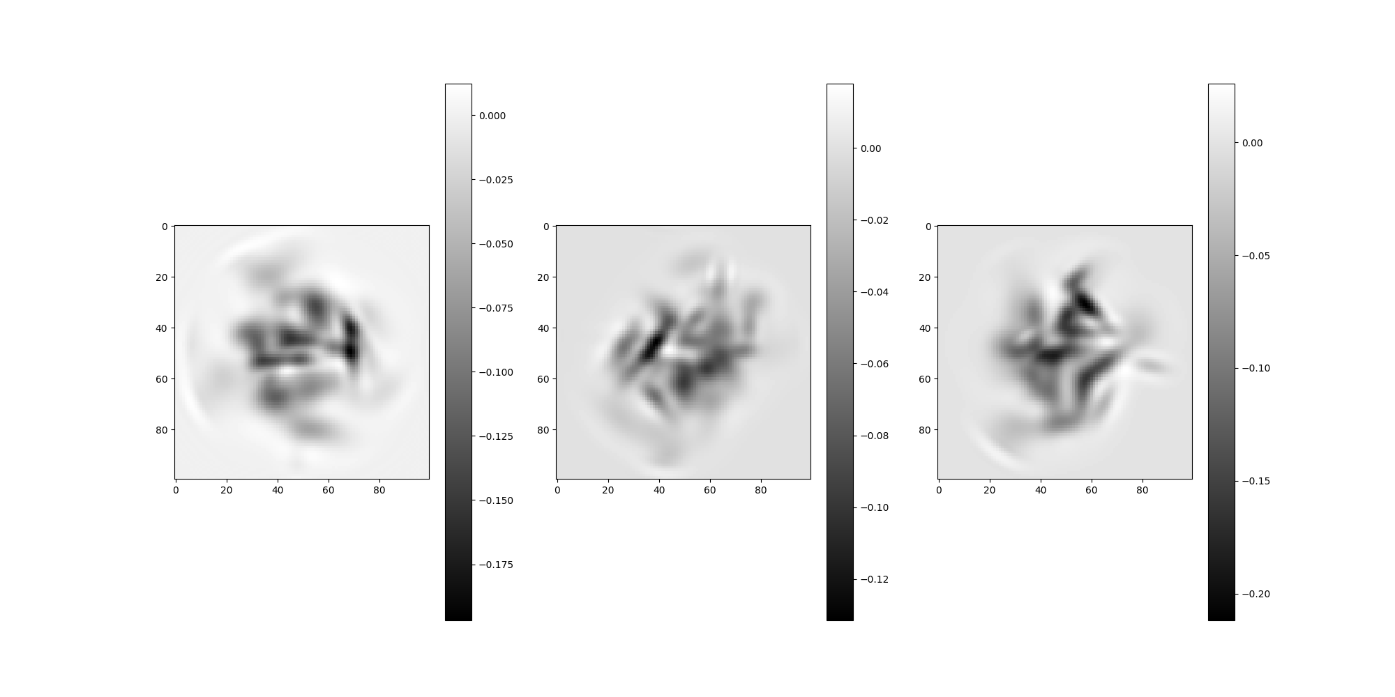
Let’s find the images from the Simulation using the get_particle_indices method to retrieve their global indices.

global_particle_indices = np.zeros((n_particles), dtype=int)
for i in range(n_particles):
    global_particle_indices[i] = src.get_particle_indices(
        test_micrograph, local_particle_indices[i]
    )

# Plot the simulation's images
src.simulation.images[global_particle_indices].show()

We can check if these global indices match our local particle indices with the get_micrograph_index method.

check_local_indices = np.zeros((n_particles), dtype=int)
for i in range(n_particles):
    # Get each particle's corresponding micrograph index and local particle index
    micrograph_index, check_local_indices[i] = src.get_micrograph_index(
        global_particle_indices[i]
    )
    assert micrograph_index == 1
np.testing.assert_array_equal(local_particle_indices, check_local_indices)
print(f"Local particle indices: {check_local_indices}")

Local particle indices: [24 20 36]

Saving a MicrographSimulation

In addition to saving the raw MRC files, MicrographSimulation populates STAR files with the particle centers, particle box size (rlnImageSize), and projection rotations. Additionally, CTF parameters are saved when CTF is used in the simulation. Each micrograph will have a corresponidng STAR file. The collection of these files are returned from MicrographSimulation.save as a list of tuples which is designed to work directly with CentersCoordinateSource.

from aspire.source import CentersCoordinateSource

# Save the simulation
results = src.save(os.path.join(tmp_dir.name, "mg_sim"))

# Review the resulting files
print(results)

[('/tmp/tmpqm4jr7r8/mg_sim/micrograph_0.mrc', '/tmp/tmpqm4jr7r8/mg_sim/micrograph_0.star'), ('/tmp/tmpqm4jr7r8/mg_sim/micrograph_1.mrc', '/tmp/tmpqm4jr7r8/mg_sim/micrograph_1.star'), ('/tmp/tmpqm4jr7r8/mg_sim/micrograph_2.mrc', '/tmp/tmpqm4jr7r8/mg_sim/micrograph_2.star')]

# Review the example STAR file contents
with open(results[0][1], "r") as f:
    print(f.read())

data_
loop_
_rlnImageName
_rlnImageSize
_rlnCoordinateX
_rlnCoordinateY
_rlnAngleRot
_rlnAngleTilt
_rlnAnglePsi
_rlnVoltage
_rlnDefocusU
_rlnDefocusV
_rlnDefocusAngle
_rlnSphericalAberration
_rlnAmplitudeContrast
000001@micrograph_0 100 357 514 225.17323 70.42997 85.89395 200.0 15000.0 15000.0 0.0 2.26 0.07
000002@micrograph_0 100 118 467 67.95413 99.76551 37.444767 200.0 15000.0 15000.0 0.0 2.26 0.07
000003@micrograph_0 100 590 277 7.2576475 140.38687 300.22638 200.0 15000.0 15000.0 0.0 2.26 0.07
000004@micrograph_0 100 522 248 63.480827 84.10157 7.4896197 200.0 15000.0 15000.0 0.0 2.26 0.07
000005@micrograph_0 100 223 745 229.15794 21.15329 197.15344 200.0 15000.0 15000.0 0.0 2.26 0.07
000006@micrograph_0 100 174 445 260.969 149.42964 175.6943 200.0 15000.0 15000.0 0.0 2.26 0.07
000007@micrograph_0 100 299 59 47.95209 136.74622 193.82863 200.0 15000.0 15000.0 0.0 2.26 0.07
000008@micrograph_0 100 659 434 91.8869 100.16265 202.57196 200.0 15000.0 15000.0 0.0 2.26 0.07
000009@micrograph_0 100 117 647 329.64502 75.08341 13.788601 200.0 15000.0 15000.0 0.0 2.26 0.07
000010@micrograph_0 100 735 339 46.58517 129.15901 187.30682 200.0 15000.0 15000.0 0.0 2.26 0.07
000011@micrograph_0 100 491 789 110.339386 99.2707 85.04628 200.0 15000.0 15000.0 0.0 2.26 0.07
000012@micrograph_0 100 809 818 336.5936 52.53211 220.0516 200.0 15000.0 15000.0 0.0 2.26 0.07
000013@micrograph_0 100 436 431 134.82375 125.791466 127.273315 200.0 15000.0 15000.0 0.0 2.26 0.07
000014@micrograph_0 100 212 212 88.836 131.61661 170.09749 200.0 15000.0 15000.0 0.0 2.26 0.07
000015@micrograph_0 100 374 937 71.1484 50.87036 117.835976 200.0 15000.0 15000.0 0.0 2.26 0.07
000016@micrograph_0 100 159 101 63.209724 61.319878 215.21576 200.0 15000.0 15000.0 0.0 2.26 0.07
000017@micrograph_0 100 727 717 171.41907 103.669914 162.73087 200.0 15000.0 15000.0 0.0 2.26 0.07
000018@micrograph_0 100 434 566 148.2073 23.667522 192.28221 200.0 15000.0 15000.0 0.0 2.26 0.07
000019@micrograph_0 100 514 940 124.225586 101.704155 352.64386 200.0 15000.0 15000.0 0.0 2.26 0.07
000020@micrograph_0 100 644 172 242.63022 54.44209 61.728706 200.0 15000.0 15000.0 0.0 2.26 0.07
000021@micrograph_0 100 758 943 197.08356 43.91972 100.298325 200.0 15000.0 15000.0 0.0 2.26 0.07
000022@micrograph_0 100 394 628 359.41455 75.2847 220.48091 200.0 15000.0 15000.0 0.0 2.26 0.07
000023@micrograph_0 100 87 144 171.61751 15.32889 111.023254 200.0 15000.0 15000.0 0.0 2.26 0.07
000024@micrograph_0 100 204 235 326.69586 57.931633 271.72266 200.0 15000.0 15000.0 0.0 2.26 0.07
000025@micrograph_0 100 775 436 24.332895 108.68852 9.214272 200.0 15000.0 15000.0 0.0 2.26 0.07
000026@micrograph_0 100 702 85 166.2759 55.460697 243.91948 200.0 15000.0 15000.0 0.0 2.26 0.07
000027@micrograph_0 100 816 257 342.33093 164.46213 154.5533 200.0 15000.0 15000.0 0.0 2.26 0.07
000028@micrograph_0 100 245 494 205.81186 160.12997 93.87625 200.0 15000.0 15000.0 0.0 2.26 0.07
000029@micrograph_0 100 222 116 39.215176 119.0958 321.86478 200.0 15000.0 15000.0 0.0 2.26 0.07
000030@micrograph_0 100 499 733 108.81932 61.365723 181.91663 200.0 15000.0 15000.0 0.0 2.26 0.07
000031@micrograph_0 100 947 736 109.85279 42.58259 210.66025 200.0 15000.0 15000.0 0.0 2.26 0.07
000032@micrograph_0 100 134 621 36.03223 105.68081 324.1332 200.0 15000.0 15000.0 0.0 2.26 0.07
000033@micrograph_0 100 106 707 312.10165 33.21698 55.839603 200.0 15000.0 15000.0 0.0 2.26 0.07
000034@micrograph_0 100 233 487 336.63525 81.33271 271.0917 200.0 15000.0 15000.0 0.0 2.26 0.07
000035@micrograph_0 100 576 110 79.40814 74.74897 337.01068 200.0 15000.0 15000.0 0.0 2.26 0.07
000036@micrograph_0 100 439 755 267.8921 65.83309 255.31674 200.0 15000.0 15000.0 0.0 2.26 0.07
000037@micrograph_0 100 395 504 204.60135 136.76486 181.031 200.0 15000.0 15000.0 0.0 2.26 0.07
000038@micrograph_0 100 738 721 47.220955 58.597233 144.94357 200.0 15000.0 15000.0 0.0 2.26 0.07
000039@micrograph_0 100 952 243 78.088165 78.69344 2.2200234 200.0 15000.0 15000.0 0.0 2.26 0.07
000040@micrograph_0 100 631 543 220.26422 161.4182 308.45044 200.0 15000.0 15000.0 0.0 2.26 0.07
000041@micrograph_0 100 903 635 317.36963 141.55984 150.86116 200.0 15000.0 15000.0 0.0 2.26 0.07
000042@micrograph_0 100 599 527 276.6933 48.701714 132.33043 200.0 15000.0 15000.0 0.0 2.26 0.07
000043@micrograph_0 100 215 962 188.79645 59.49243 256.79306 200.0 15000.0 15000.0 0.0 2.26 0.07
000044@micrograph_0 100 120 455 274.22302 16.362684 58.064697 200.0 15000.0 15000.0 0.0 2.26 0.07
000045@micrograph_0 100 135 738 183.78815 115.328545 255.8863 200.0 15000.0 15000.0 0.0 2.26 0.07
000046@micrograph_0 100 937 717 356.82742 117.60184 176.06554 200.0 15000.0 15000.0 0.0 2.26 0.07
000047@micrograph_0 100 71 684 257.85233 63.155346 49.60995 200.0 15000.0 15000.0 0.0 2.26 0.07
000048@micrograph_0 100 644 568 130.81349 123.28017 78.281044 200.0 15000.0 15000.0 0.0 2.26 0.07
000049@micrograph_0 100 672 915 146.05128 137.0732 329.7856 200.0 15000.0 15000.0 0.0 2.26 0.07
000050@micrograph_0 100 130 103 86.410545 123.06443 121.30503 200.0 15000.0 15000.0 0.0 2.26 0.07

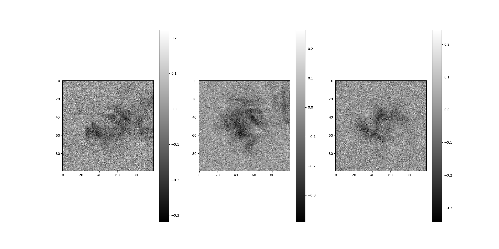
img_src = CentersCoordinateSource(results, src.particle_box_size)
# Show the first five images from the image source.
img_src.images[:3].show()

# Cleanup the tmp_dir
tmp_dir.cleanup()