Basic Image Array

In this example we will demonstrate some of ASPIRE’s image processing functionality. We will add noise to a stack of copies of a stock image. We will then estimate and whiten that noise using some tools from the ASPIRE pipeline.

import matplotlib.pyplot as plt
import numpy as np
from scipy.datasets import face

from aspire.image import Image
from aspire.noise import AnisotropicNoiseEstimator, CustomNoiseAdder, WhiteNoiseAdder
from aspire.operators import FunctionFilter
from aspire.source import ArrayImageSource

Stock Image

Lets get some basic image data as a numpy array. Scipy ships with a portrait.

# We'll take the grayscale representation as floating point data.
stock_img = face(gray=True).astype(np.float32)

# Crop to a square
n_pixels = min(stock_img.shape)
stock_img = stock_img[0:n_pixels, 0:n_pixels]
# Normalize to [0,1]
stock_img /= np.max(stock_img)

Add Noise to the Image

Now that we have an example array, we will begin using the ASPIRE toolkit. First we will make an ASPIRE Image instance out of our data. This is a light wrapper over the numpy array. Many ASPIRE internals are built around an Image class.

# Construct the Image class by passing it an array of data.
img = Image(stock_img)
# Downsample (just to speeds things up)
new_resolution = img.resolution // 4
img = img.downsample(new_resolution)


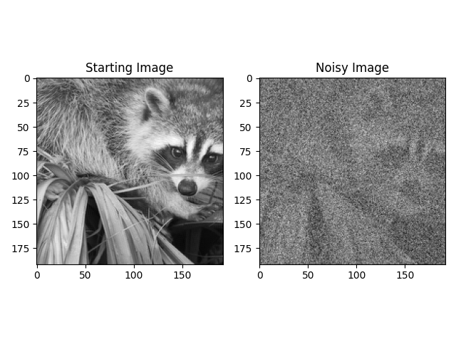
# We will begin processing by adding some noise.
# We would like to create uniform noise for a 2d image with prescibed variance,
noise_var = np.var(img.asnumpy()) * 5

# Then create a WhiteNoiseAdder.
noise = WhiteNoiseAdder(var=noise_var, seed=123)

# We can apply the WhiteNoiseAdder to our image data.
img_with_noise = noise.forward(img)

# We will plot the original and first noisy image,
# because we only have one image in our Image stack right now.
fig, axs = plt.subplots(1, 2)
axs[0].imshow(img.asnumpy()[0], cmap=plt.cm.gray)
axs[0].set_title("Starting Image")
axs[1].imshow(img_with_noise.asnumpy()[0], cmap=plt.cm.gray)
axs[1].set_title("Noisy Image")
plt.tight_layout()
plt.show()

Adding Noise to a Simulated Stack of Images

Great, now we have enough to try an experiment. This time we will use a stack of images. In real use, you would probably bring your own array of images, or use a Simulation object. For now we’ll create some arrays as before. For demonstration we’ll setup a stack of n_imgs, with each image just being a copy of the data from img.

n_imgs = 128
imgs_data = np.empty((n_imgs, img.resolution, img.resolution), dtype=np.float64)
for i in range(n_imgs):
    imgs_data[i] = img[0]
imgs = Image(imgs_data)


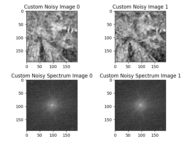
# Lets say we want to add different kind of noise to the images.
# We can create our own function. Here we want to apply in two dimensions.
def noise_function(x, y):
    return np.exp(-(x * x + y * y) / (2 * 0.3**2))


# We can create a custom filter from that function.
f = FunctionFilter(noise_function)
# And use the filter to add the noise to our stack of images.
noise_adder = CustomNoiseAdder(noise_filter=f, seed=123)
imgs_with_noise = noise_adder.forward(imgs)

# Let's see the first two noisy images.
# They should each display slightly different noise.
fig, axs = plt.subplots(2, 2)
for i, img in enumerate(imgs_with_noise[0:2].asnumpy()):
    axs[0, i].imshow(img, cmap=plt.cm.gray)
    axs[0, i].set_title(f"Custom Noisy Image {i}")
    img_with_noise_f = np.abs(np.fft.fftshift(np.fft.fft2(img)))
    axs[1, i].imshow(np.log(1 + img_with_noise_f), cmap=plt.cm.gray)
    axs[1, i].set_title(f"Custom Noisy Spectrum Image {i}")
plt.tight_layout()
plt.show()

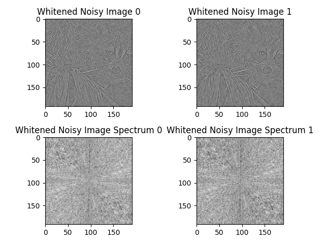
Noise Estimation and Whitening

Now we will use an ASPIRE pipeline to whiten the image stack. Here we will introduce our Source class and demonstrate applying an Xform.

# ``Source`` classes are what we use in processing pipelines.
# They provide a consistent interface to a variety of underlying data sources.
# In this case, we'll just use our Image in an ArrayImageSource to run a small experiment.
#
# If you were happy with the experiment design on an array of test data,
# the source is easily swapped out to something like RelionSource,
# which might point at a stack of images too large to fit in memory at once.
# The implementation of batching for memory management
# would be managed behind the scenes for you.

imgs_src = ArrayImageSource(imgs_with_noise)

# We'll copy the orginals for comparison later, before we process them further.
noisy_imgs_copy = imgs_src.images[:n_imgs].asnumpy()

# One of the tools we can use is a NoiseEstimator,
#   which consumes from a Source.
noise_estimator = AnisotropicNoiseEstimator(imgs_src)

# Once we have the estimator instance,
#   we can use it in a transform applied to our Source.
imgs_src = imgs_src.whiten(noise_estimator)


# Peek at two whitened images and their corresponding spectrum.
fig, axs = plt.subplots(2, 2)
for i, img in enumerate(imgs_src.images[:2].asnumpy()):
    axs[0, i].imshow(img, cmap=plt.cm.gray)
    axs[0, i].set_title(f"Whitened Noisy Image {i}")
    img_with_noise_f = np.abs(np.fft.fftshift(np.fft.fft2(img)))
    axs[1, i].imshow(np.log(1 + img_with_noise_f), cmap=plt.cm.gray)
    axs[1, i].set_title(f"Whitened Noisy Image Spectrum {i}")
plt.tight_layout()
plt.show()

  0%|          | 0/1 [00:00<?, ?it/s]
100%|██████████| 1/1 [00:00<00:00,  5.15it/s]
100%|██████████| 1/1 [00:00<00:00,  5.14it/s]

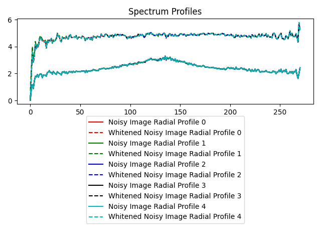
Power Spectral Density

We will also want to take a look at the power spectral density. Since we just want to see the character of what is happening, We will assume each pixel’s contribution is placed at its lower left corner, and compute a crude radial profile. Code from a discussion at https://stackoverflow.com/questions/21242011/most-efficient-way-to-calculate-radial-profile.

def radial_profile(data):
    y, x = np.indices((data.shape))
    # Distance from origin to lower left corner
    r = np.sqrt(x**2 + y**2).astype(int)
    binsum = np.bincount(r.ravel(), np.log(1 + data.ravel()))
    bincount = np.bincount(r.ravel())
    # Return the mean per bin
    return binsum / bincount


# Lets pickout several images and plot their the radial profile of their noise.
colors = ["r", "g", "b", "k", "c"]
for i, img in enumerate(imgs_src.images[: len(colors)].asnumpy()):
    img_with_noise_f = np.abs(np.fft.fftshift(np.fft.fft2(noisy_imgs_copy[i])))
    plt.plot(
        radial_profile(img_with_noise_f),
        color=colors[i],
        label=f"Noisy Image Radial Profile {i}",
    )

    whitened_img_with_noise_f = np.abs(np.fft.fftshift(np.fft.fft2(img)))
    plt.plot(
        radial_profile(whitened_img_with_noise_f),
        color=colors[i],
        linestyle="--",
        label=f"Whitened Noisy Image Radial Profile {i}",
    )

plt.title("Spectrum Profiles")
plt.gca().legend(loc="upper center", bbox_to_anchor=(0.5, -0.1))
plt.tight_layout()
plt.show()