2D Covariance Estimation

This script illustrates 2D covariance Wiener filtering functionality in the ASPIRE package, implemented by estimating the covariance of the unfiltered images in a Fourier-Bessel basis and applying the Wiener filter induced by that covariance matrix.

import logging
import os

import matplotlib.pyplot as plt
import numpy as np

from aspire.basis import FFBBasis2D
from aspire.covariance import RotCov2D
from aspire.noise import WhiteNoiseAdder
from aspire.operators import RadialCTFFilter
from aspire.source.simulation import Simulation
from aspire.utils import anorm
from aspire.volume import Volume

logger = logging.getLogger(__name__)

file_path = os.path.join(
    os.path.dirname(os.getcwd()), "data", "clean70SRibosome_vol_65p.mrc"
)


logger.info(
    "This script illustrates 2D covariance Wiener filtering functionality in ASPIRE package."
)

Image Formatting

# Set the sizes of images 64 x 64
img_size = 64
# Set the total number of images generated from the 3D map
num_imgs = 1024
# Set dtype for this experiment
dtype = np.float32
logger.info(f"Simulation running in {dtype} precision.")

Build Noise Filter

Set the noise variance and build the noise filter It might be better to select a signal noise ratio and initial noise inside the Simulation class.

noise_var = 1.3957e-4
noise_adder = WhiteNoiseAdder(var=noise_var)

Specify the CTF Parameters

pixel_size = 5 * 65 / img_size  # Pixel size of the images (in angstroms)
voltage = 200  # Voltage (in KV)
defocus_min = 1.5e4  # Minimum defocus value (in angstroms)
defocus_max = 2.5e4  # Maximum defocus value (in angstroms)
defocus_ct = 7  # Number of defocus groups.
Cs = 2.0  # Spherical aberration
alpha = 0.1  # Amplitude contrast

Initialize Simulation Object and CTF Filters

logger.info("Initialize simulation object and CTF filters.")
# Create filters
ctf_filters = [
    RadialCTFFilter(pixel_size, voltage, defocus=d, Cs=2.0, alpha=0.1)
    for d in np.linspace(defocus_min, defocus_max, defocus_ct)
]

# Load the map file of a 70S Ribosome
logger.info(
    f"Load 3D map and downsample 3D map to desired grids "
    f"of {img_size} x {img_size} x {img_size}."
)
vols = Volume.load(file_path, dtype=dtype)

# Scale and downsample
vols[0] /= np.max(vols[0])
vols = vols.downsample(img_size)

# Create a simulation object with specified filters and the downsampled 3D map
logger.info("Use downsampled map to creat simulation object.")
sim = Simulation(
    L=img_size,
    n=num_imgs,
    vols=vols,
    unique_filters=ctf_filters,
    offsets=0.0,
    amplitudes=1.0,
    dtype=dtype,
    noise_adder=noise_adder,
)

Build Clean and Noisy Projection Images

# Specify the fast FB basis method for expanding the 2D images
ffbbasis = FFBBasis2D((img_size, img_size), dtype=dtype)

# Assign the CTF information and index for each image
h_idx = sim.filter_indices

# Evaluate CTF in the 8X8 FB basis
h_ctf_fb = [ffbbasis.filter_to_basis_mat(filt) for filt in ctf_filters]

# Get clean images from projections of 3D map.
logger.info("Apply CTF filters to clean images.")
imgs_clean = sim.projections[:]
imgs_ctf_clean = sim.clean_images[:]
power_clean = imgs_ctf_clean.norm() ** 2 / imgs_ctf_clean.size
sn_ratio = power_clean / noise_var
logger.info(f"Signal to noise ratio is {sn_ratio}.")

# get noisy images after applying CTF and noise filters
imgs_noise = sim.images[:num_imgs]

Expand Images in the Fourier-Bessel Basis

Expand the images, both clean and noisy, in the Fourier-Bessel basis. This can be done exactly (that is, up to numerical precision) using the basis.expand function, but for our purposes, an approximation will do. Since the basis is close to orthonormal, we may approximate the exact expansion by applying the adjoint of the evaluation mapping using basis.evaluate_t.

logger.info("Get coefficients of clean and noisy images in FFB basis.")
coef_clean = ffbbasis.evaluate_t(imgs_clean)
coef_noise = ffbbasis.evaluate_t(imgs_noise)

Create Cov2D Object and Calculate Mean and Variance for Clean Images

Create the Cov2D object and calculate mean and covariance for clean images without CTF. Given the clean Fourier-Bessel coefficients, we can estimate the symmetric mean and covariance. Note that these are not the same as the sample mean and covariance, since these functions use the rotational and reflectional symmetries of the distribution to constrain to further constrain the estimate. Note that the covariance matrix estimate is not a full matrix, but is block diagonal. This form is a consequence of the symmetry constraints, so to reduce space, only the diagonal blocks are stored. The mean and covariance estimates will allow us to evaluate the mean and covariance estimates from the filtered, noisy data, later.

logger.info(
    "Get 2D covariance matrices of clean and noisy images using FB coefficients."
)
cov2d = RotCov2D(ffbbasis)
mean_coef = cov2d.get_mean(coef_clean)
covar_coef = cov2d.get_covar(coef_clean, mean_coef, noise_var=0)

Estimate mean and covariance for noisy images with CTF and shrink method

We now estimate the mean and covariance from the Fourier-Bessel coefficients of the noisy, filtered images. These functions take into account the filters applied to each image to undo their effect on the estimates. For the covariance estimation, the additional information of the estimated mean and the variance of the noise are needed. Again, the covariance matrix estimate is provided in block diagonal form.

covar_opt = {
    "shrinker": "frobenius_norm",
    "verbose": 0,
    "max_iter": 250,
    "iter_callback": [],
    "store_iterates": False,
    "rel_tolerance": 1e-12,
    "precision": "float64",
    "preconditioner": "identity",
}
mean_coef_est = cov2d.get_mean(coef_noise, h_ctf_fb, h_idx)
covar_coef_est = cov2d.get_covar(
    coef_noise,
    h_ctf_fb,
    h_idx,
    mean_coef_est,
    noise_var=noise_var,
    covar_est_opt=covar_opt,
)

Estimate Fourier-Bessel Coefficients with Wiener Filter

Estimate the Fourier-Bessel coefficients of the underlying images using a Wiener filter. This Wiener filter is calculated from the estimated mean, covariance, and the variance of the noise. The resulting estimator has the lowest expected mean square error out of all linear estimators.

logger.info("Get the CWF coefficients of noising images.")
coef_est = cov2d.get_cwf_coefs(
    coef_noise,
    h_ctf_fb,
    h_idx,
    mean_coef=mean_coef_est,
    covar_coef=covar_coef_est,
    noise_var=noise_var,
)

# Convert Fourier-Bessel coefficients back into 2D images
imgs_est = ffbbasis.evaluate(coef_est)

Evaluate the Results

# Calculate the difference between the estimated covariance and the "true"
# covariance estimated from the clean Fourier-Bessel coefficients.
covar_coef_diff = covar_coef - covar_coef_est

# Calculate the deviation between the clean estimates and those obtained from
# the noisy, filtered images.
diff_mean = anorm(mean_coef_est - mean_coef) / anorm(mean_coef)
diff_covar = covar_coef_diff.norm() / covar_coef.norm()

# Calculate the normalized RMSE of the estimated images.
nrmse_ims = (imgs_est - imgs_clean).norm() / imgs_clean.norm()
logger.info(f"Deviation of the noisy mean estimate: {diff_mean}")
logger.info(f"Deviation of the noisy covariance estimate: {diff_covar}")
logger.info(f"Estimated images normalized RMSE: {nrmse_ims}")

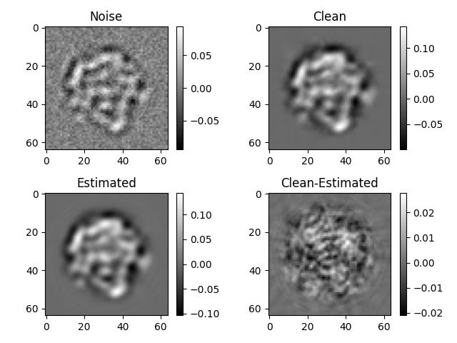
# plot the first images at different stages
idm = 0
plt.subplot(2, 2, 1)
plt.imshow(-imgs_noise.asnumpy()[idm], cmap="gray")
plt.colorbar()
plt.title("Noise")
plt.subplot(2, 2, 2)
plt.imshow(imgs_clean.asnumpy()[idm], cmap="gray")
plt.colorbar()
plt.title("Clean")
plt.subplot(2, 2, 3)
plt.imshow(imgs_est.asnumpy()[idm], cmap="gray")
plt.colorbar()
plt.title("Estimated")
plt.subplot(2, 2, 4)
plt.imshow(imgs_est.asnumpy()[idm] - imgs_clean.asnumpy()[idm], cmap="gray")
plt.colorbar()
plt.title("Clean-Estimated")
plt.tight_layout()

# Basic Check
assert nrmse_ims < 0.25