Image Preprocessing

This script illustrates the preprocess steps implemented prior to starting the pipeline of reconstructing a 3D map using simulated 2D images.

import logging
import os

import matplotlib.pyplot as plt
import numpy as np

from aspire.noise import WhiteNoiseAdder
from aspire.operators import RadialCTFFilter
from aspire.source.simulation import Simulation
from aspire.volume import Volume

logger = logging.getLogger(__name__)

file_path = os.path.join(
    os.path.dirname(os.getcwd()), "data", "clean70SRibosome_vol_65p.mrc"
)

Specify Parameters

# Set the initial simulated full size of images.
img_size = 33

# Set the demonstration downsampled image size.
ds_img_size = 15

# Set the total number of images generated from the 3D map
num_imgs = 512

# Set the noise variance and build the noise filter
noise_variance = 4e-1
noise_adder = WhiteNoiseAdder(var=noise_variance)

# Specify the CTF parameters not used for this example
# but necessary for initializing the simulation object
pixel_size = 5 * 65 / img_size  # Pixel size of the images (in angstroms)
voltage = 200  # Voltage (in KV)
defocus_min = 1.5e4  # Minimum defocus value (in angstroms)
defocus_max = 2.5e4  # Maximum defocus value (in angstroms)
defocus_ct = 7  # Number of defocus groups
Cs = 2.0  # Spherical aberration
alpha = 0.1  # Amplitude contrast

Build Simulation Object and Apply Noise

logger.info("Initialize simulation object and CTF filters.")
# Create CTF filters
ctf_filters = [
    RadialCTFFilter(pixel_size, voltage, defocus=d, Cs=2.0, alpha=0.1)
    for d in np.linspace(defocus_min, defocus_max, defocus_ct)
]

# Load the map file of a 70S ribosome and downsample the 3D map to desired image size.
logger.info("Load 3D map from mrc file")
vols = Volume.load(file_path)

# Downsample the volume to a desired image size and increase density
# by 1.0e5 time for a better graph view
logger.info(f"Downsample map to a image size of {img_size} x {img_size} x {img_size}")
vols = vols.downsample(img_size) * 1.0e5

# Create a simulation object with specified filters and the downsampled 3D map
logger.info("Use downsampled map to create simulation object.")
source = Simulation(
    L=img_size,
    n=num_imgs,
    vols=vols,
    unique_filters=ctf_filters,
    noise_adder=noise_adder,
)

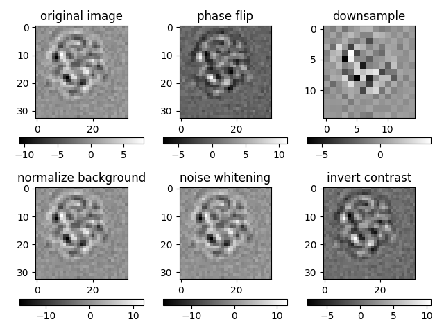
Apply Independent Preprocessing Techniques

Now we’ll apply each technique sequentially. This is easily accomplished because each preprocessing technique returns a new ImageSource object. In this case we assign each to a new variable source_*. That leaves the original source object untouched.

logger.info("Obtain original images.")
imgs_od = source.images[0].asnumpy()

logger.info("Perform phase flip to input images.")
source_pf = source.phase_flip()

logger.info(f"Downsample image size to {ds_img_size} X {ds_img_size}")
source_ds = source.downsample(ds_img_size)

logger.info("Normalize images to background noise.")
source_nb = source.normalize_background()

logger.info("Whiten noise of images")
source_wt = source.whiten()

logger.info("Invert the global density contrast if need")
source_rc = source.invert_contrast()

  0%|          | 0/1 [00:00<?, ?it/s]
100%|██████████| 1/1 [00:00<00:00,  1.13it/s]
100%|██████████| 1/1 [00:00<00:00,  1.13it/s]

  0%|          | 0/1 [00:00<?, ?it/s]
100%|██████████| 1/1 [00:00<00:00,  1.12it/s]
100%|██████████| 1/1 [00:00<00:00,  1.12it/s]

Plot First Image from Each Preprocess Step

Plot the first images.

logger.info("Plot first image from each preprocess steps")
idm = 0
plt.subplot(2, 3, 1)
plt.imshow(imgs_od[idm], cmap="gray")
plt.colorbar(orientation="horizontal")
plt.title("original image")

plt.subplot(2, 3, 2)
plt.imshow(source_pf.images[0].asnumpy()[idm], cmap="gray")
plt.colorbar(orientation="horizontal")
plt.title("phase flip")

plt.subplot(2, 3, 3)
plt.imshow(source_ds.images[0].asnumpy()[idm], cmap="gray")
plt.colorbar(orientation="horizontal")
plt.title("downsample")

plt.subplot(2, 3, 4)
plt.imshow(source_nb.images[0].asnumpy()[idm], cmap="gray")
plt.colorbar(orientation="horizontal")
plt.title("normalize background")

plt.subplot(2, 3, 5)
plt.imshow(source_wt.images[0].asnumpy()[idm], cmap="gray")
plt.colorbar(orientation="horizontal")
plt.title("noise whitening")

plt.subplot(2, 3, 6)
plt.imshow(source_rc.images[0].asnumpy()[idm], cmap="gray")
plt.colorbar(orientation="horizontal")
plt.title("invert contrast")
plt.tight_layout()

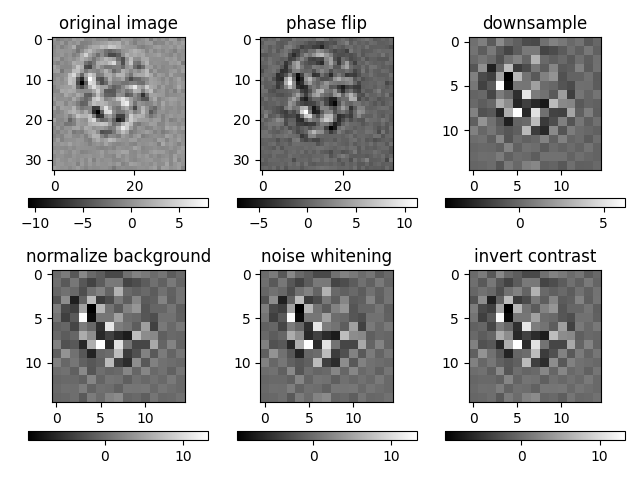
Apply Sequential Preprocessing Techniques

Now we’ll apply each technique sequentially. This is accomplished by reassigning each new ImageSource to the same variable. In this case we reassign to source. Note, after each source assignment we’ll manually save off the images for the plot below.

# We'll copy ``source`` so we can use it in a later section.
# Since ``source`` objects are designed to follow an immutable usage by default (like Numpy arrays),
# we can copy a source just by copying the object.
source_copy = source

logger.info("Obtain original images.")
imgs_seq_od = source.images[0].asnumpy()

logger.info("Perform phase flip to input images.")
source = source.phase_flip()
imgs_seq_pf = source.images[0].asnumpy()

logger.info(f"Downsample image size to {ds_img_size} X {ds_img_size}")
source = source.downsample(ds_img_size)
imgs_seq_ds = source.images[0].asnumpy()

logger.info("Normalize images to background noise.")
source = source.normalize_background()
imgs_seq_nb = source.images[0].asnumpy()

logger.info("Whiten noise of images")
source = source.whiten()
imgs_seq_wt = source.images[0].asnumpy()

logger.info("Invert the global density contrast if need")
source = source.invert_contrast()
imgs_seq_rc = source.images[0].asnumpy()

  0%|          | 0/1 [00:00<?, ?it/s]
100%|██████████| 1/1 [00:00<00:00,  1.09it/s]
100%|██████████| 1/1 [00:00<00:00,  1.09it/s]

  0%|          | 0/1 [00:00<?, ?it/s]
100%|██████████| 1/1 [00:00<00:00,  1.05it/s]
100%|██████████| 1/1 [00:00<00:00,  1.05it/s]

Plot First Image from Each Preprocess Step

Plot the first images.

logger.info("Plot first image from each preprocess steps")
idm = 0
plt.subplot(2, 3, 1)
plt.imshow(imgs_od[idm], cmap="gray")
plt.colorbar(orientation="horizontal")
plt.title("original image")

plt.subplot(2, 3, 2)
plt.imshow(imgs_seq_pf[idm], cmap="gray")
plt.colorbar(orientation="horizontal")
plt.title("phase flip")

plt.subplot(2, 3, 3)
plt.imshow(imgs_seq_ds[idm], cmap="gray")
plt.colorbar(orientation="horizontal")
plt.title("downsample")

plt.subplot(2, 3, 4)
plt.imshow(imgs_seq_nb[idm], cmap="gray")
plt.colorbar(orientation="horizontal")
plt.title("normalize background")

plt.subplot(2, 3, 5)
plt.imshow(imgs_seq_wt[idm], cmap="gray")
plt.colorbar(orientation="horizontal")
plt.title("noise whitening")

plt.subplot(2, 3, 6)
plt.imshow(imgs_seq_rc[idm], cmap="gray")
plt.colorbar(orientation="horizontal")
plt.title("invert contrast")
plt.tight_layout()

Apply Chained Preprocessing Techniques

Now we’ll apply the preprocessing in a chain syntax

# We'll reset our ``source`` to the reference copy we started with.
source = source_copy

logger.info("Perform phase flip to input images.")
logger.info(f"Downsample image size to {ds_img_size} X {ds_img_size}")
logger.info("Normalize images to background noise.")
logger.info("Whiten noise of images")
logger.info("Invert the global density contrast if need")
source = (
    source.phase_flip()
    .downsample(ds_img_size)
    .normalize_background()
    .whiten()
    .invert_contrast()
)
# Assign the first image from the preprocessed chain.
imgs_chained = source.images[0].asnumpy()

# This preprocessing chain should correspond to applying each
# operation sequentially.
assert np.allclose(imgs_chained, imgs_seq_rc)

  0%|          | 0/1 [00:00<?, ?it/s]
100%|██████████| 1/1 [00:00<00:00,  1.07it/s]
100%|██████████| 1/1 [00:00<00:00,  1.07it/s]

  0%|          | 0/1 [00:00<?, ?it/s]
100%|██████████| 1/1 [00:01<00:00,  1.03s/it]
100%|██████████| 1/1 [00:01<00:00,  1.03s/it]