Relion Projection Interoperability

In this tutorial we compare projections generated by Relion with projections generated by ASPIRE’s Simulation class. Both sets of projections are generated using a downsampled volume map of a 70S Ribosome, absent of noise and CTF corruption.

import os

import numpy as np

from aspire.source import RelionSource, Simulation
from aspire.volume import Volume

Load Relion Projections

We load the Relion projections as a RelionSource and view the images.

starfile = os.path.join(os.path.dirname(os.getcwd()), "data", "rln_proj_65.star")
rln_src = RelionSource(starfile)
rln_src.images[:].show(colorbar=False)

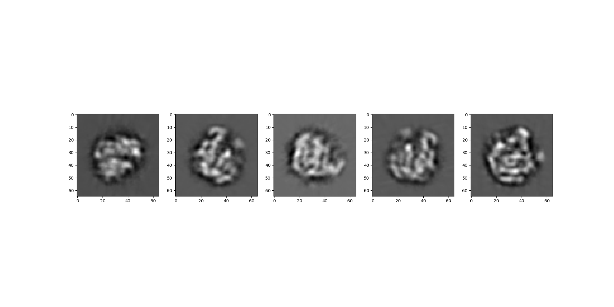
Note

The projections above were generated in Relion using the following command:

relion_project --i clean70SRibosome_vol_65p.mrc --nr_uniform 3000 --angpix 5

For this tutorial we take a subset of these projections consisting of the first 5 images.

Generate Projections using Simulation

Using the metadata associated with the RelionSource and the same volume we generate an analogous set of projections with ASPIRE’s Simulation class.

# Load the volume from file as a ``Volume`` object.
filepath = os.path.join(
    os.path.dirname(os.getcwd()), "data", "clean70SRibosome_vol_65p.mrc"
)
vol = Volume.load(filepath, dtype=rln_src.dtype)

# Create a ``Simulation`` source using metadata from the RelionSource projections.
# Note, for odd resolution Relion projections are shifted from ASPIRE projections
# by 1 pixel in x and y.
sim_src = Simulation(
    n=rln_src.n,
    vols=vol,
    offsets=-np.ones((rln_src.n, 2), dtype=rln_src.dtype),
    amplitudes=rln_src.amplitudes,
    angles=rln_src.angles,
    dtype=rln_src.dtype,
)

sim_src.images[:].show(colorbar=False)

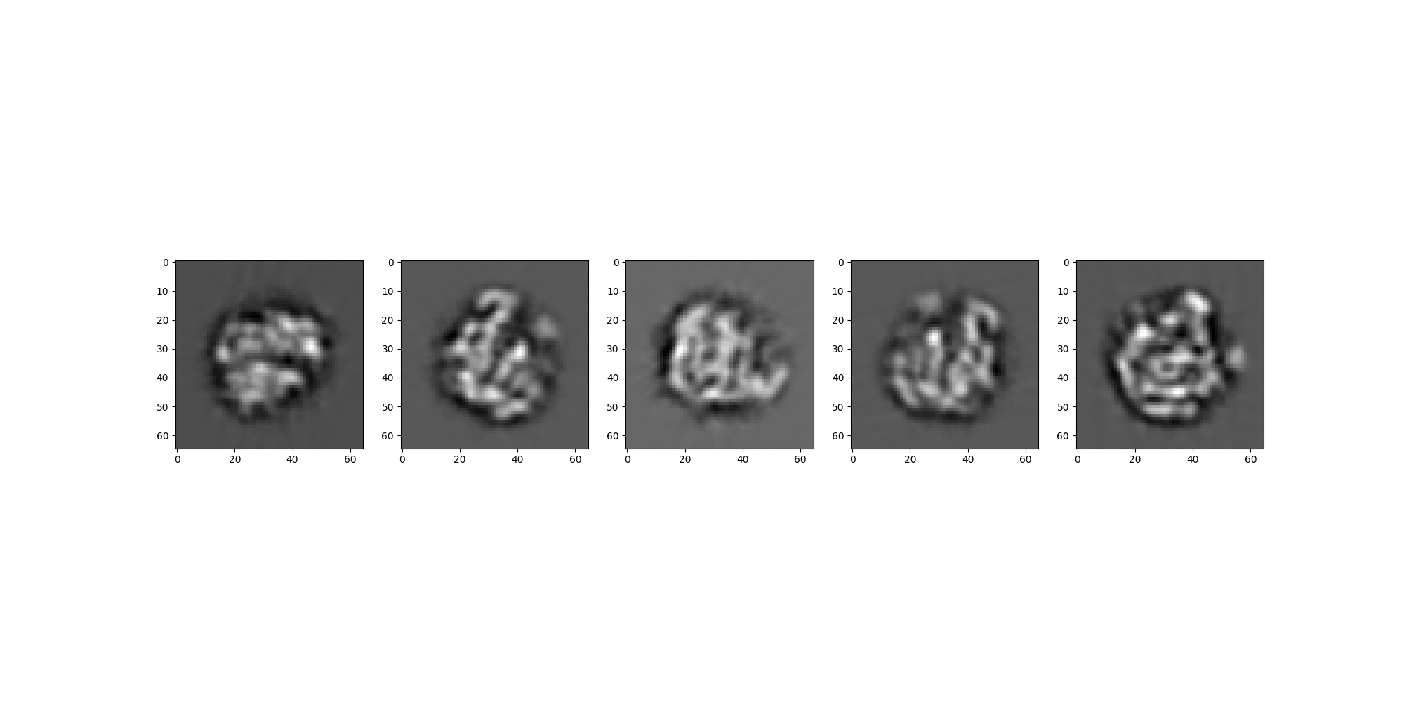
Comparing the Projections

We will take a few different approaches to comparing the two sets of projection images.

Visual Comparison

We’ll first look at a side-by-side of the two sets of images to confirm visually that the projections are taken from the same viewing angles.

rln_src.images[:].show(colorbar=False)
sim_src.images[:].show(colorbar=False)

• 
• 

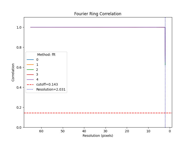
Fourier Ring Correlation

Additionally, we can compare the two sets of images using the FRC. Note that the images are tightly correlated up to a high resolution of 2 pixels.

rln_src.images[:].frc(sim_src.images[:], cutoff=0.143, plot=True)

(array([2.03125, 2.03125, 2.03125, 2.03125, 2.03125]), array([[0.9999512 , 0.9997589 , 0.99972236, 0.9997412 , 0.9998079 ,
        0.9996844 , 0.99985576, 0.9998627 , 0.9996016 , 0.9998016 ,
        0.99976003, 0.99937594, 0.9995311 , 0.9995893 , 0.9993813 ,
        0.99957883, 0.9996111 , 0.99948037, 0.9995136 , 0.9994557 ,
        0.9994089 , 0.99950975, 0.999424  , 0.99937224, 0.99928445,
        0.9991797 , 0.99939245, 0.99923795, 0.9991501 , 0.9988561 ,
        0.99914384, 0.6890389 ],
       [0.99996084, 0.9996519 , 0.99941367, 0.9996295 , 0.99953634,
        0.9997356 , 0.99981254, 0.999729  , 0.99975413, 0.99976027,
        0.99978626, 0.9996996 , 0.9996597 , 0.99939144, 0.99957305,
        0.99935323, 0.99950606, 0.9995502 , 0.99923104, 0.9994775 ,
        0.9993991 , 0.9992754 , 0.99930483, 0.9992679 , 0.99936   ,
        0.99925387, 0.99918777, 0.99928516, 0.9992362 , 0.99918747,
        0.9990527 , 0.6563474 ],
       [0.99980867, 0.9999284 , 0.99962634, 0.99976695, 0.99972266,
        0.99960023, 0.99968237, 0.9997462 , 0.99980867, 0.9996951 ,
        0.99984986, 0.9996864 , 0.9996273 , 0.99971586, 0.9995882 ,
        0.9995541 , 0.99949145, 0.9993193 , 0.9991364 , 0.99951273,
        0.9994654 , 0.9995991 , 0.9994171 , 0.99944943, 0.9992521 ,
        0.9989504 , 0.99913013, 0.9994102 , 0.9994244 , 0.9992472 ,
        0.9988976 , 0.6197828 ],
       [0.99984056, 0.9997645 , 0.9996911 , 0.9998639 , 0.9996305 ,
        0.9997983 , 0.9997752 , 0.99962395, 0.9997876 , 0.99984217,
        0.9998592 , 0.9996771 , 0.9994766 , 0.99927455, 0.9995294 ,
        0.99945295, 0.99952775, 0.99958897, 0.99937934, 0.999444  ,
        0.9995143 , 0.99963874, 0.9994448 , 0.9992456 , 0.99928594,
        0.9992858 , 0.9989985 , 0.9992831 , 0.99888504, 0.9988116 ,
        0.9988935 , 0.7134864 ],
       [0.99992067, 0.99977815, 0.9996207 , 0.99962646, 0.99944603,
        0.9997416 , 0.9997854 , 0.99961793, 0.9997694 , 0.9998145 ,
        0.99977046, 0.99975216, 0.9997679 , 0.9995889 , 0.99926215,
        0.9995358 , 0.9994929 , 0.99951744, 0.9996956 , 0.999419  ,
        0.9994483 , 0.999326  , 0.99935865, 0.9993657 , 0.99932224,
        0.9992338 , 0.9994343 , 0.99917585, 0.9990704 , 0.99915725,
        0.9991647 , 0.6540188 ]], dtype=float32))

Relative Error

As Relion and ASPIRE differ in methods of generating projections, the pixel intensity of the images may not correspond perfectly. So we begin by first normalizing the two sets of projections. We then check that the relative error with respect to the frobenius norm is less than 3%.

# Work with numpy arrays.
rln_np = rln_src.images[:].asnumpy()
sim_np = sim_src.images[:].asnumpy()

# Normalize images.
rln_np = (rln_np - np.mean(rln_np)) / np.std(rln_np)
sim_np = (sim_np - np.mean(sim_np)) / np.std(sim_np)

# Assert that error is less than 3%.
error = np.linalg.norm(rln_np - sim_np, axis=(1, 2)) / np.linalg.norm(
    rln_np, axis=(1, 2)
)
assert all(error < 0.03)
print(f"Relative per-image error: {error}")

Relative per-image error: [0.02434895 0.02776893 0.02810042 0.02241797 0.02729611]