Note
Go to the end to download the full example code.
Class Averaging
We demonstrate class averaging using the rotationally invariant representation algorithm.
import matplotlib.pyplot as plt
import numpy as np
from PIL import Image as PILImage

from aspire.denoising import DebugClassAvgSource, DefaultClassAvgSource
from aspire.noise import WhiteNoiseAdder
from aspire.source import ArrayImageSource  # Helpful hint if you want to BYO array.
from aspire.utils import gaussian_2d
Build Simulated Data
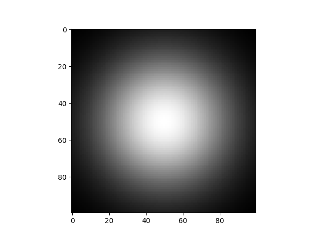
Circular 2D Gaussian Image
L = 100
round_disc = gaussian_2d(L, sigma=L / 4)
plt.imshow(round_disc, cmap="gray")
plt.show()
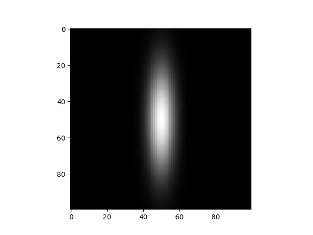
Oval 2D Gaussian Image
oval_disc = gaussian_2d(L, sigma=(L / 20, L / 5))
plt.imshow(oval_disc, cmap="gray")
plt.show()
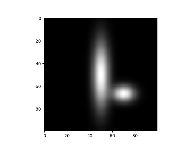
Handed Image
Create richer test set by including an asymmetric image.
# Create a second oval.
oval_disc2 = gaussian_2d(L, mu=(L / 5, L / 6), sigma=(L / 15, L / 20))

# Strategically add it to `oval_disc`.
yoval_discL = oval_disc.copy()
yoval_discL += oval_disc2
plt.imshow(yoval_discL, cmap="gray")
plt.show()
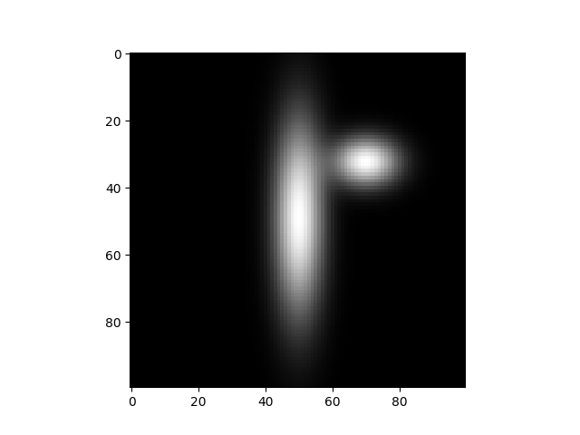
Reflected Image
Also include the reflection of the asymmetric image.
yoval_discR = np.flipud(yoval_discL)
plt.imshow(yoval_discR, cmap="gray")
plt.show()
Example Data Set Source
We concatenate and shuffle 512 rotations of the Gaussian images above to create our data set.
# How many entries (angles) in our stack
N = 512
thetas = np.linspace(start=0, stop=360, num=N, endpoint=False)

classRound = np.zeros((N, L, L))
classOval = np.zeros((N, L, L))
classYOvalL = np.zeros((N, L, L))
classYOvalR = np.zeros((N, L, L))

for i, theta in enumerate(thetas):
    classRound[i] = np.asarray(PILImage.fromarray(round_disc).rotate(theta))
    classOval[i] = np.asarray(PILImage.fromarray(oval_disc).rotate(theta))
    classYOvalL[i] = np.asarray(PILImage.fromarray(yoval_discL).rotate(theta))
    classYOvalR[i] = np.asarray(PILImage.fromarray(yoval_discR).rotate(theta))

# We'll make an example data set by concatentating then shuffling
# these.
example_array = np.concatenate((classRound, classOval, classYOvalL, classYOvalR))
np.random.seed(1234567)
np.random.shuffle(example_array)

# So now that we have cooked up an example dataset, lets create an
# ASPIRE source
src = ArrayImageSource(example_array, pixel_size=1.0)

# Let's peek at the images to make sure they're shuffled up nicely
src.images[:10].show()

Basic Class Average
This first example uses the DebugClassAvgSource to classify
images via the rotationally invariant representation
(RIRClass2D) algorithm. DebugClassAvgSource internally uses
TopClassSelector by default. TopClassSelector
deterministically selects the first n_classes.
DebugClassAvgSource also uses brute force rotational alignment
without shifts. These simplifications are useful for development
and debugging. Later we will discuss the more general
ClassAvgSource and the modular components that are more suitable
to simulations and experimental datasets.
avgs = DebugClassAvgSource(
    src=src,
    n_nbor=10,
)
Display Classes
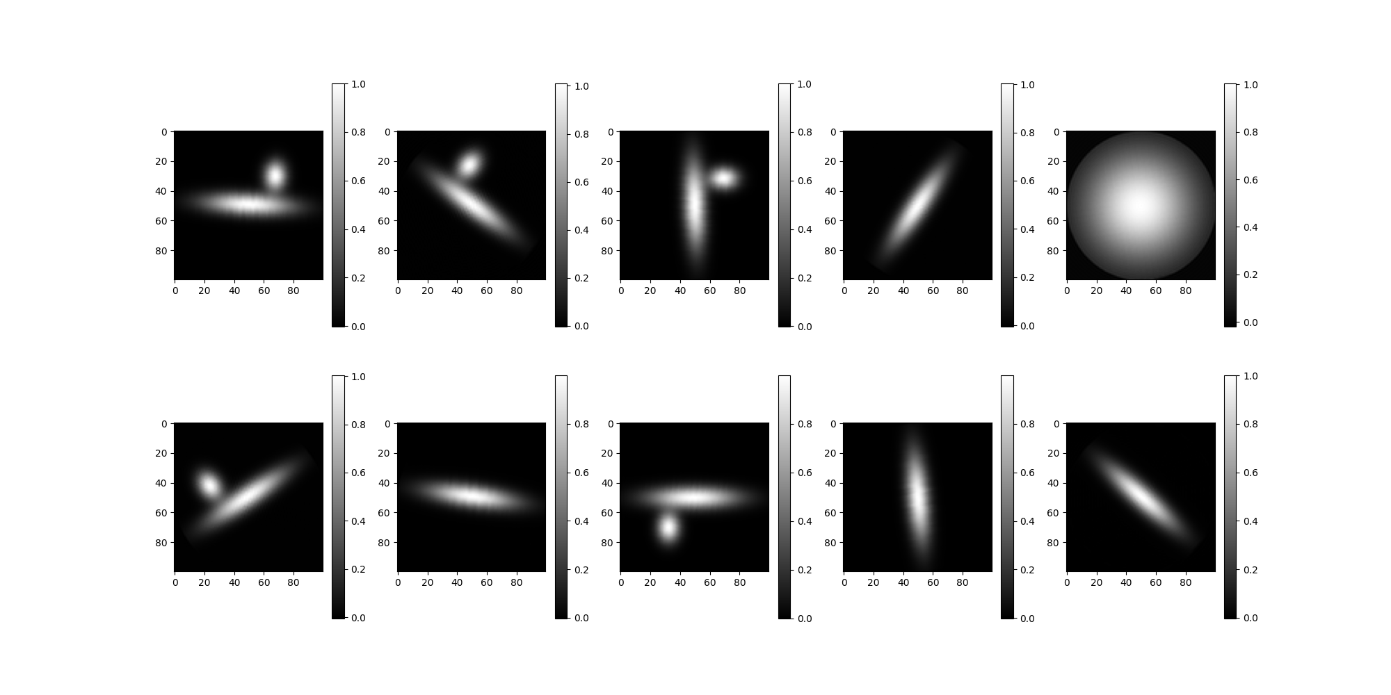
Now we will request the first 10 images and display them.
avgs.images[:10].show()
  0%|          | 0/4 [00:00<?, ?it/s]
 75%|███████▌  | 3/4 [00:00<00:00, 23.45it/s]
100%|██████████| 4/4 [00:00<00:00, 23.26it/s]

  0%|          | 0/4 [00:00<?, ?it/s]
 25%|██▌       | 1/4 [00:00<00:00,  9.56it/s]
 50%|█████     | 2/4 [00:00<00:00,  9.67it/s]
100%|██████████| 4/4 [00:00<00:00,  9.86it/s]
100%|██████████| 4/4 [00:00<00:00,  9.81it/s]

Rotationally aligning classes:   0%|          | 0/10 [00:00<?, ?it/s]
Rotationally aligning classes:  20%|██        | 2/10 [00:00<00:00,  9.32it/s]
Rotationally aligning classes:  30%|███       | 3/10 [00:00<00:00,  9.15it/s]
Rotationally aligning classes:  40%|████      | 4/10 [00:00<00:00,  8.43it/s]
Rotationally aligning classes:  50%|█████     | 5/10 [00:00<00:00,  7.75it/s]
Rotationally aligning classes:  60%|██████    | 6/10 [00:00<00:00,  7.52it/s]
Rotationally aligning classes:  70%|███████   | 7/10 [00:00<00:00,  8.06it/s]
Rotationally aligning classes:  80%|████████  | 8/10 [00:00<00:00,  8.20it/s]
Rotationally aligning classes:  90%|█████████ | 9/10 [00:01<00:00,  7.91it/s]


Stacking and evaluating batch of class averages from FFBBasis2D to Cartesian:   0%|          | 0/1 [00:00<?, ?it/s]

Stacking batch:   0%|          | 0/10 [00:00<?, ?it/s]

Stacking batch:  20%|██        | 2/10 [00:00<00:00, 16.08it/s]

Stacking batch:  60%|██████    | 6/10 [00:00<00:00, 28.05it/s]

Stacking batch: 100%|██████████| 10/10 [00:00<00:00, 32.90it/s]


Stacking and evaluating batch of class averages from FFBBasis2D to Cartesian: 100%|██████████| 1/1 [00:00<00:00,  2.83it/s]
Class Averaging with Noise
Add Noise to Data Set
# Using the sample variance, we'll compute a target noise variance
# Noise
var = np.var(src.images[:].asnumpy())
noise_var = var * 2**4

# Then create noise with the ``WhiteNoiseAdder`` class.
noise = WhiteNoiseAdder(var=noise_var, seed=123)

# Add noise to the images by performing ``forward``
noisy_im = noise.forward(src.images[:])

# Recast as an ASPIRE source
noisy_src = ArrayImageSource(noisy_im)

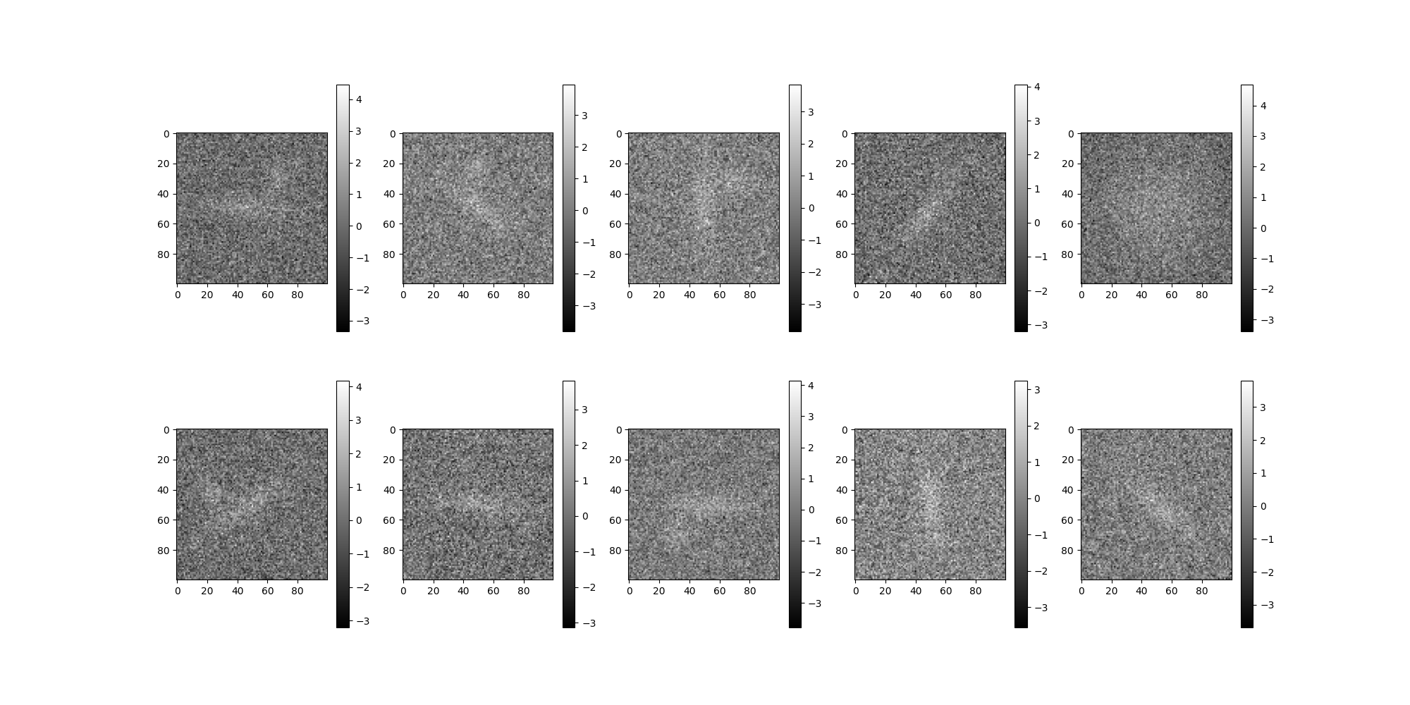
# Let's peek at the noisey images
noisy_src.images[:10].show()
RIR with Noise
Here we will use the noise_src.
avgs = DebugClassAvgSource(
    src=noisy_src,
    n_nbor=10,
)
Display Classes
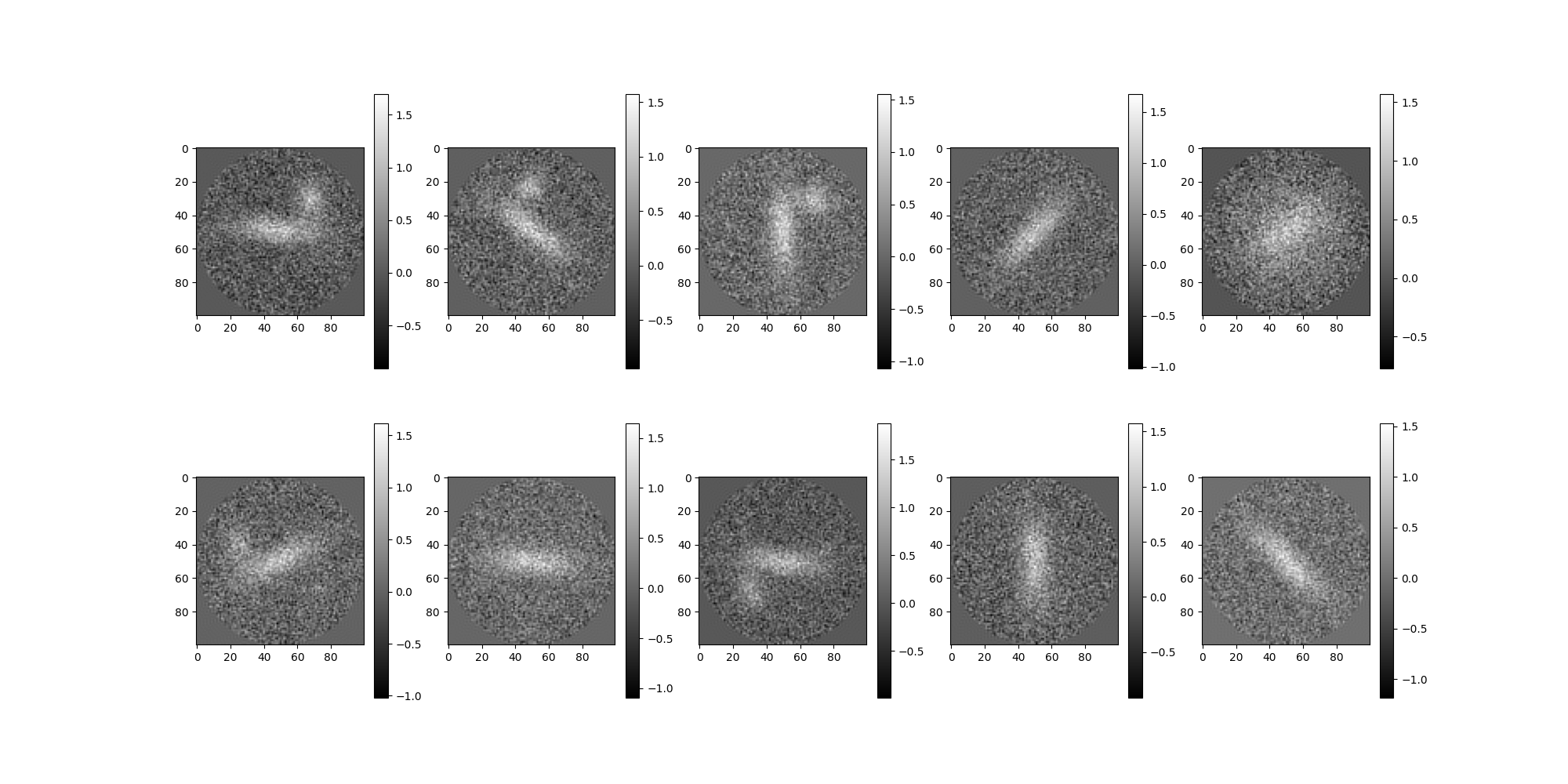
Here, on request for images, the class average source will classify,
select, and average images. All this occurs inside the
ClassAvgSource components. When using more advanced class
average sources, the images are remapped by the selector. In this
case, using DebugClassAvgSource the first 10 images will simply
correspond to the first ten from noise_src.
avgs.images[:10].show()
  0%|          | 0/4 [00:00<?, ?it/s]
 75%|███████▌  | 3/4 [00:00<00:00, 21.18it/s]
100%|██████████| 4/4 [00:00<00:00, 21.37it/s]

  0%|          | 0/4 [00:00<?, ?it/s]
 50%|█████     | 2/4 [00:00<00:00, 13.03it/s]
100%|██████████| 4/4 [00:00<00:00, 13.66it/s]
100%|██████████| 4/4 [00:00<00:00, 13.55it/s]

Rotationally aligning classes:   0%|          | 0/10 [00:00<?, ?it/s]
Rotationally aligning classes:  10%|█         | 1/10 [00:00<00:01,  8.92it/s]
Rotationally aligning classes:  20%|██        | 2/10 [00:00<00:01,  6.23it/s]
Rotationally aligning classes:  30%|███       | 3/10 [00:00<00:01,  6.53it/s]
Rotationally aligning classes:  40%|████      | 4/10 [00:00<00:00,  7.11it/s]
Rotationally aligning classes:  50%|█████     | 5/10 [00:00<00:00,  7.36it/s]
Rotationally aligning classes:  60%|██████    | 6/10 [00:00<00:00,  6.81it/s]
Rotationally aligning classes:  70%|███████   | 7/10 [00:01<00:00,  6.96it/s]
Rotationally aligning classes:  80%|████████  | 8/10 [00:01<00:00,  7.30it/s]
Rotationally aligning classes:  90%|█████████ | 9/10 [00:01<00:00,  7.59it/s]
Rotationally aligning classes: 100%|██████████| 10/10 [00:01<00:00,  7.71it/s]


Stacking and evaluating batch of class averages from FFBBasis2D to Cartesian:   0%|          | 0/1 [00:00<?, ?it/s]

Stacking batch:   0%|          | 0/10 [00:00<?, ?it/s]

Stacking batch:  20%|██        | 2/10 [00:00<00:00, 16.82it/s]

Stacking batch:  60%|██████    | 6/10 [00:00<00:00, 29.21it/s]

Stacking batch: 100%|██████████| 10/10 [00:00<00:00, 33.70it/s]


Stacking and evaluating batch of class averages from FFBBasis2D to Cartesian: 100%|██████████| 1/1 [00:00<00:00,  2.83it/s]
Review a class
Select a class to review in the output.
review_class = 5

# Map this image from the sorted selection back to the input
# ``noisy_src``.

# Report the identified neighbor indices with respect to the input
# ``noise_src``.
classes = avgs.class_indices[review_class]
reflections = avgs.class_refl[review_class]
print(f"Class {review_class}'s neighbors: {classes}")
print(f"Class {review_class}'s reflections: {reflections}")

# The original image is the initial image in the class array.
original_image_idx = classes[0]
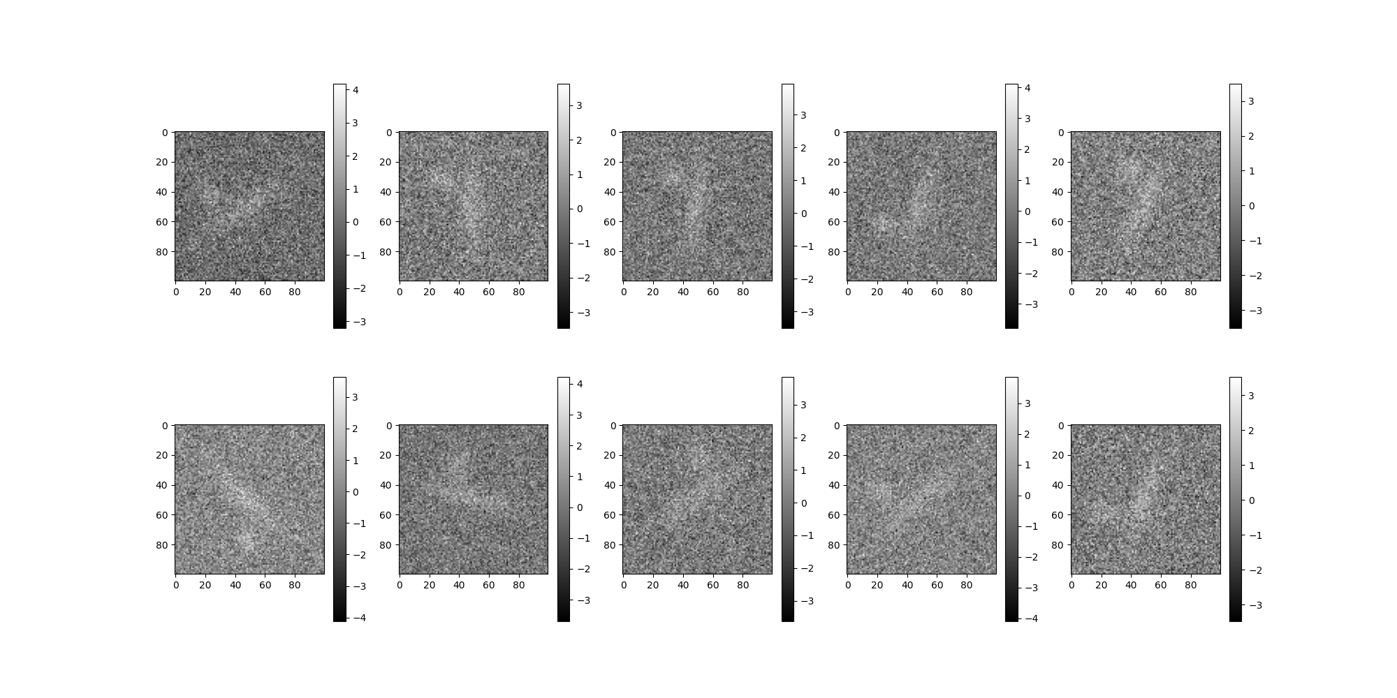
Class 5's neighbors: [   5 1746 1894 1218 1170 1307 1829  313  441 1621]
Class 5's reflections: [False  True  True  True  True False False False False False]
Report the identified neighbors, original is the first image.
noisy_src.images[classes].show()
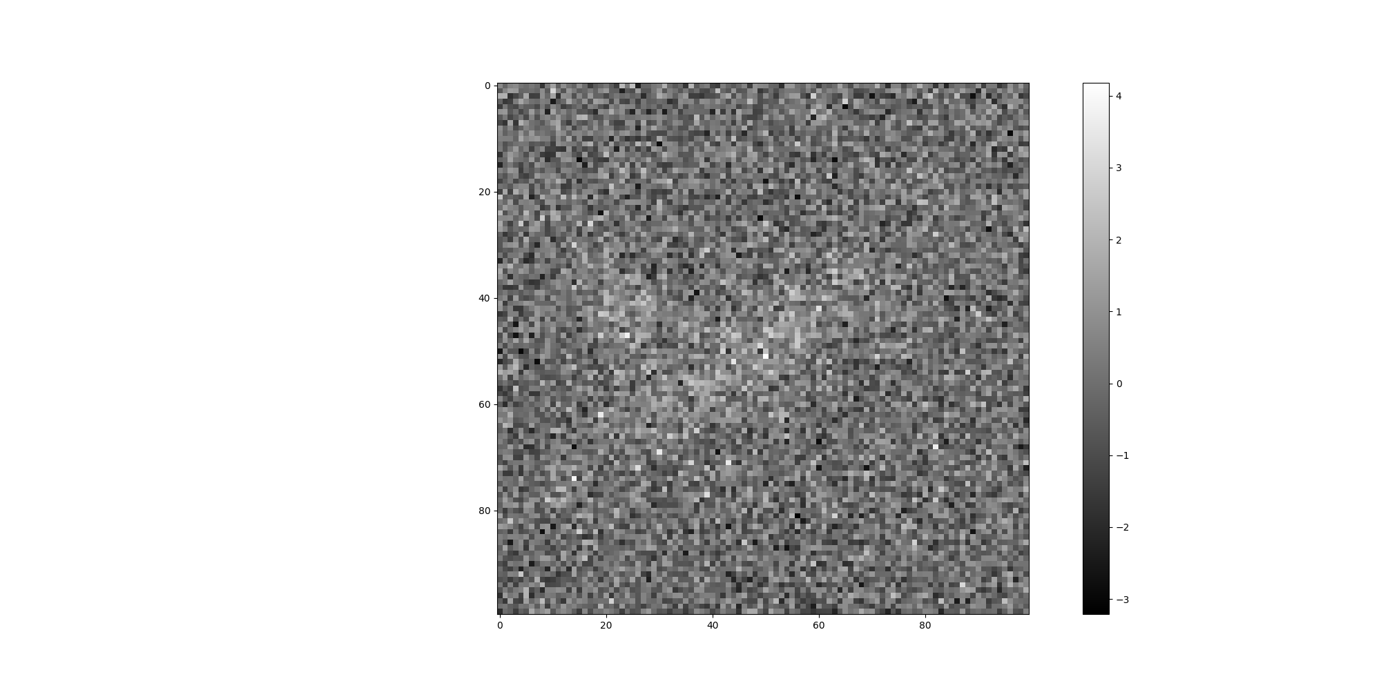
Display original image.
noisy_src.images[original_image_idx].show()
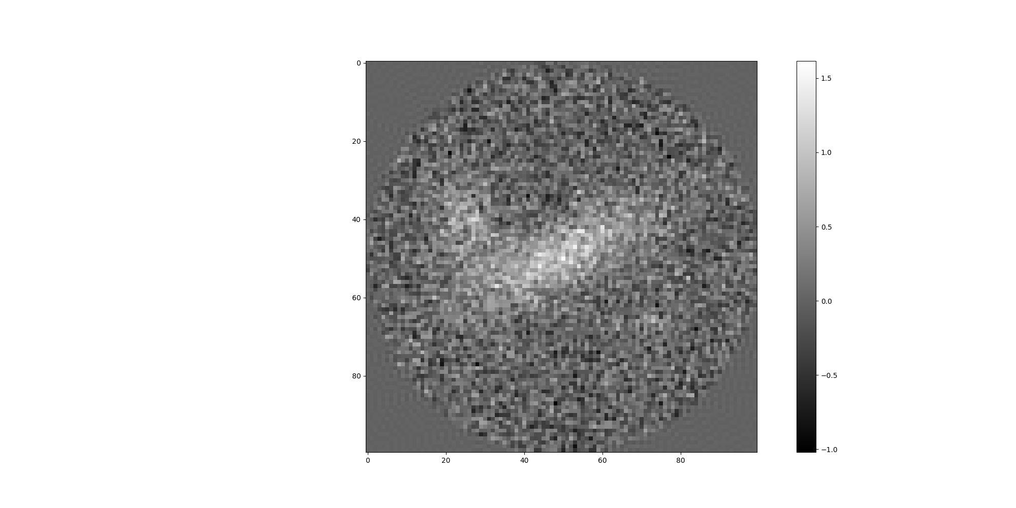
Display the averaged result
avgs.images[review_class].show()
Rotationally aligning classes:   0%|          | 0/1 [00:00<?, ?it/s]
Rotationally aligning classes: 100%|██████████| 1/1 [00:00<00:00,  9.27it/s]


Stacking and evaluating batch of class averages from FFBBasis2D to Cartesian:   0%|          | 0/1 [00:00<?, ?it/s]

Stacking batch:   0%|          | 0/1 [00:00<?, ?it/s]


Stacking and evaluating batch of class averages from FFBBasis2D to Cartesian: 100%|██████████| 1/1 [00:00<00:00,  9.07it/s]
Alignment Details
Alignment details are exposed when available from an underlying
averager. In this case, we’ll get the estimated alignments for
the review_class.
est_rotations = avgs.averager.rotations
est_shifts = avgs.averager.shifts
est_dot_products = avgs.averager.dot_products

# These are dictionaries mapping each class to arrays of attributes.
print(f"Estimated Rotations: {est_rotations}")
print(f"Estimated Shifts: {est_shifts}")
print(f"Estimated Dot Products: {est_dot_products}")

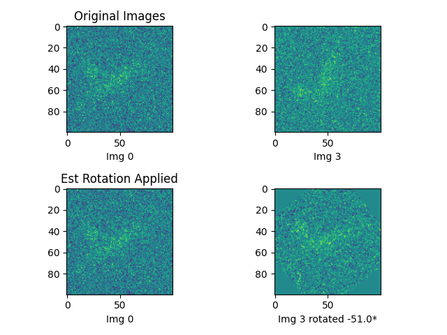
# Compare the original unaligned images with the estimated alignment.
# Get the indices from the classification results.
nbr = 3
original_img_0_idx = classes[0]
original_img_nbr_idx = classes[nbr]

# Lookup the images.
original_img_0 = noisy_src.images[original_img_0_idx].asnumpy()[0]
original_img_nbr = noisy_src.images[original_img_nbr_idx].asnumpy()[0]

# Rotate using estimated rotations.
# First retrieve all angles for the `review_class` (original_img_0_idx),
#   then lookup the specific neighbor `nbr`
assert (
    original_img_0_idx == review_class
), "DebugClassAvgSource should retain original source image ordering"
angle = est_rotations[original_img_0_idx][nbr] * 180 / np.pi
if reflections[nbr]:
    print("Reflection reported.")
    original_img_nbr = np.flipud(original_img_nbr)
rotated_img_nbr = np.asarray(PILImage.fromarray(original_img_nbr).rotate(angle))

plt.subplot(2, 2, 1)
plt.title("Original Images")
plt.imshow(original_img_0)
plt.xlabel("Img 0")
plt.subplot(2, 2, 2)
plt.imshow(original_img_nbr)
plt.xlabel(f"Img {nbr}")

plt.subplot(2, 2, 3)
plt.title("Est Rotation Applied")
plt.imshow(original_img_0)
plt.xlabel("Img 0")
plt.subplot(2, 2, 4)
plt.imshow(rotated_img_nbr)
plt.xlabel(f"Img {nbr} rotated {angle:.4}*")
plt.tight_layout()
plt.show()
Estimated Rotations: {np.int64(0): array([-0.        , -5.34070751, -5.20108117, -2.68780705, -2.04203522,
       -0.54105207, -2.39110108, -0.85521133, -5.84685299, -0.43633231]), np.int64(1): array([-0.        , -5.06145483, -2.75762022, -3.70009801, -1.01229097,
       -2.12930169, -2.19911486, -1.1693706 , -1.65806279, -2.72271363]), np.int64(2): array([-0.        , -5.3756141 , -4.81710874, -0.31415927, -5.3581608 ,
       -3.97935069, -1.46607657, -6.14355897, -0.4712389 , -5.88175958]), np.int64(3): array([-0.        , -4.95673508, -4.38077642, -1.67551608, -3.21140582,
       -3.70009801, -4.59021593, -1.29154365, -4.99164166, -5.56760031]), np.int64(4): array([-0.        , -5.30580093, -3.90953752, -1.09955743, -3.59537826,
       -3.12413936, -2.28638132, -4.53785606, -1.43116999, -1.72787596]), np.int64(5): array([-0.        , -1.09955743, -4.9043752 , -1.11701072, -0.06981317,
       -0.34906585, -5.21853446, -5.41052068, -3.47320521, -1.97222205]), np.int64(6): array([-0.        , -2.11184839, -1.22173048, -5.06145483, -6.0562925 ,
       -0.20943951, -2.42600766, -5.79449312, -1.1693706 , -3.17649924]), np.int64(7): array([-0.        , -2.84488668, -3.97935069, -0.61086524, -3.47320521,
       -0.        , -0.        , -3.17649924, -2.89724656, -0.08726646]), np.int64(8): array([-0.        , -4.11897703, -5.39306739, -2.93215314, -4.34586984,
       -5.18362788, -2.98451302, -3.4906585 , -5.51524044, -2.51327412]), np.int64(9): array([-0.        , -4.59021593, -0.15707963, -4.03171057, -5.8293997 ,
       -1.58824962, -3.71755131, -2.77507351, -5.61996019, -1.76278254])}
Estimated Shifts: {}
Estimated Dot Products: {np.int64(0): array([5865.9046832 ,  546.4922547 ,  579.91263458,  475.63008507,
        583.52409409,  517.87511085,  533.39155275,  534.5179154 ,
        538.2218787 ,  477.5037366 ]), np.int64(1): array([6005.39865871,  627.39764773,  569.494419  ,  511.74579838,
        483.61749048,  594.87288006,  551.52043353,  510.73442242,
        598.46310764,  568.29438291]), np.int64(2): array([6102.66048713,  593.79585344,  561.12652611,  572.6665563 ,
        540.75995694,  554.01073063,  516.10634697,  680.94191362,
        573.92624548,  616.28385805]), np.int64(3): array([5888.48157466,  428.42103216,  449.02148132,  501.23035634,
        433.04205626,  481.85646342,  455.13585619,  482.37726453,
        468.03261539,  534.79808318]), np.int64(4): array([7438.81431202,  781.33129204, 2136.64841687,  717.50443875,
        803.43082695, 2104.71966681,  904.94324935, 2160.4078535 ,
       2192.78258646,  579.20590903]), np.int64(5): array([5852.89921803,  573.28999826,  479.46088919,  519.78865321,
        524.99186463,  516.02695266,  580.33586184,  587.87430859,
        480.90882755,  594.50869367]), np.int64(6): array([5858.86172826,  421.78750959,  709.72448386,  482.90301631,
        499.36951812,  545.52542075,  509.85799491,  449.9642986 ,
        494.21010371,  482.64031888]), np.int64(7): array([6000.98327771,  657.1408667 ,  596.71582105,  572.9711919 ,
        529.66754836,  567.80980089,  611.4786066 ,  658.55832548,
        549.18855371,  600.55895998]), np.int64(8): array([5744.94222533,  364.94150708,  470.59459865,  502.98205496,
        471.32452521,  612.4526049 ,  488.95120997,  520.34677813,
        457.16267711,  634.34296156]), np.int64(9): array([5722.08330654,  436.15759193,  427.1263987 ,  529.97986103,
        425.99846111,  437.25139008,  467.61165075,  482.57152768,
        414.83335204,  425.81817743])}
Reflection reported.
ClassAvgSource Components
For more realistic simulations and experimental data,
ASPIRE provides a wholly customizable base ClassAvgSource
class. This class expects a user to instantiate and provide
all components required for class averaging.
To make things easier a practical starting point
DefaultClassAvgSource is provided which fills in reasonable
defaults based on what is available in the current ASPIRE-Python.
The defaults can be overridden simply by instantiating your own
instances of components and passing during initialization.
# Using the defaults requires only passing a source.
# After understanding the various components that can be
# combined in a ``ClassAvgSource``, they can be customized
# or easily extended.
avg_src = DefaultClassAvgSource(noisy_src)
Total running time of the script: (0 minutes 44.968 seconds)