ASPIRE-Python Introduction

In this notebook we will introduce the core API components, then demonstrate basic usage corresponding to topics from Princeton’s MAT586.

Installation

ASPIRE can generally install on Linux, Mac, and Windows under Anaconda Python, by following the instructions in the README. The instructions for developers is the most comprehensive. Windows is provided, but generally Linux and MacOS are recommended, with Linux being the most diversely tested platform.

Princeton Research Computing

ASPIRE requires some resources to run, so if you wouldn’t run typical data science codes on your machine (a netbook for example), you may use Tiger/Adroit/Della at Princeton or another cluster. After logging into Tiger, module load anaconda3/2020.7 and continue to follow the Anaconda instructions for developers in the link above. Those instructions should create a working environment for tinkering with ASPIRE code found in this notebook.

Imports

First we import some typical scientific computing packages. Along the way we will import relevant components from aspire. Users may also import aspire once as a top level package.

import os

import matplotlib.pyplot as plt
import numpy as np

import aspire
from aspire.image import Image

API Primitives

The ASPIRE framework is a collection of modules containing interoperable extensible components. Underlying the more sophisticated components and algorithms are some core data structures. Sophisticated components are designed to interoperate by exchanging, consuming, or producing these basic structures. The most common structures encountered when starting out are:

Core API Components

Component	Description
Coef	Utility class for stacks of 1D arrays.
Image	Utility class for stacks of 2D arrays.
Volume	Utility class for stacks of 3D arrays.
Rotations	Utility class for stacks of 3D rotations.
Filter	Constructs and applies Image filters.
Basis	Basis conversions and operations.
Source	Produces primitive components. ImageSource produces Image instances.

Image Class

The Image class is a thin wrapper over Numpy arrays for a stack containing 1 or more images (2D data). In this notebook we won’t be working directly with the Image class a lot, but it will be one of the fundamental structures behind the scenes. A lot of ASPIRE code passes around Image and Volume instances.

Create an Image instance from random data.

img_data = np.random.random((100, 100))
img = Image(img_data)
print(f"img shape: {img.shape}")  # Note this produces a stack of one.
print(f"str(img): {img}")

img shape: (1, 100, 100)
str(img): 1 float64 images arranged as a (1,) stack each of size 100x100.

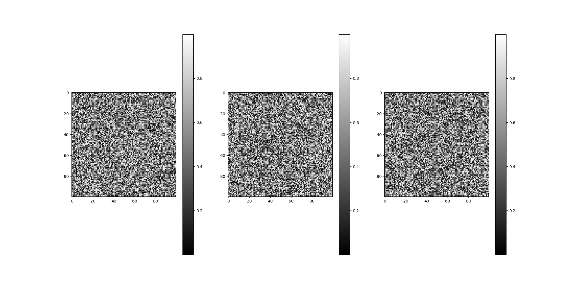
Create an Image for a stack of 3 100x100 images.

img_data = np.random.random((3, 100, 100))
img = Image(img_data)

Most often, Images will behave like Numpy arrays, but you explicitly access the underlying Numpy array via asnumpy().

img.asnumpy()

array([[[0.91678312, 0.24401413, 0.88843974, ..., 0.47951385,
         0.74978146, 0.79914219],
        [0.07196631, 0.75288803, 0.4888945 , ..., 0.6522599 ,
         0.97153285, 0.07343496],
        [0.61407588, 0.61357684, 0.89902949, ..., 0.84527926,
         0.04100338, 0.61329287],
        ...,
        [0.77212881, 0.33079248, 0.89594984, ..., 0.69387042,
         0.0524159 , 0.21834264],
        [0.37350292, 0.75355663, 0.14926636, ..., 0.56637101,
         0.06134809, 0.92902621],
        [0.42394046, 0.2473753 , 0.85899761, ..., 0.49899619,
         0.93251075, 0.73268858]],

       [[0.42921188, 0.14129711, 0.97841566, ..., 0.01653341,
         0.1981259 , 0.82613178],
        [0.83169208, 0.12973619, 0.49157156, ..., 0.22734045,
         0.15355147, 0.92412004],
        [0.82811521, 0.62724062, 0.89185085, ..., 0.85363557,
         0.1562323 , 0.25487938],
        ...,
        [0.05486182, 0.09938562, 0.33620996, ..., 0.25278208,
         0.14605589, 0.78386038],
        [0.77159439, 0.45962915, 0.36432188, ..., 0.68191564,
         0.56544489, 0.12558695],
        [0.90828933, 0.74351365, 0.75390828, ..., 0.09463541,
         0.42117929, 0.57683859]],

       [[0.33764483, 0.76195401, 0.67996366, ..., 0.28032528,
         0.6312635 , 0.16908037],
        [0.06145867, 0.67573144, 0.23019409, ..., 0.88119077,
         0.25960676, 0.91718371],
        [0.57697584, 0.74141445, 0.70386564, ..., 0.80907344,
         0.42921429, 0.85454312],
        ...,
        [0.59914649, 0.24099191, 0.44205516, ..., 0.57101082,
         0.25718563, 0.74575056],
        [0.52671529, 0.3011152 , 0.8193635 , ..., 0.4984018 ,
         0.91286054, 0.06732349],
        [0.87369312, 0.62597614, 0.21865568, ..., 0.24602644,
         0.77801477, 0.73856723]]])

Images have a built in show() method, which works well for peeking at data.

img.show()

Note

The user is responsible for using show responsibly. Avoid asking for large numbers of images that you would not normally plot. Ten or less is reasonable.

More examples using the Image class can be found in:

• ASPIRE Image Class

• Basic Image Array

Volume Class

Like Image, the Volume class is a thin wrapper over Numpy arrays that provides specialized methods for a stack containing one or more volumes (3D data).

Initialize Volume - load

A Volume may be instantiated with Numpy data similarly to Image. Both Image and Volume provide save and load methods which can be used to work with files. For Volumes .map and .mrc are currently supported. For .npy, Numpy can be used.

For example, in the following note we demonstrate instantiating an ASPIRE Volume instance using Volume.load():

Note

Instantiate an ASPIRE Volume from file:

from aspire.volume import Volume

aspire_volume = Volume.load("/path/to/volume.mrc")

In addition to the Volume.load() method, a few common starting datasets can be downloaded from EMDB using ASPIRE’s downloading utility. Below we download the high resolution volume map EMDB-2660, sourced from https://www.ebi.ac.uk/pdbe/entry/emdb/EMD-2660.

from aspire.downloader import emdb_2660

vol = emdb_2660()

Downsample Volume

Here we downsample the above volume to a desired image size (64 should be good).

img_size = 64

# Volume.downsample() returns a new Volume instance.
#   We will use this lower resolution volume later, calling it `v2`.
vol_ds = vol.downsample(img_size)
# L is often used as short hand for image and volume sizes (in pixels/voxels).
L = vol_ds.resolution

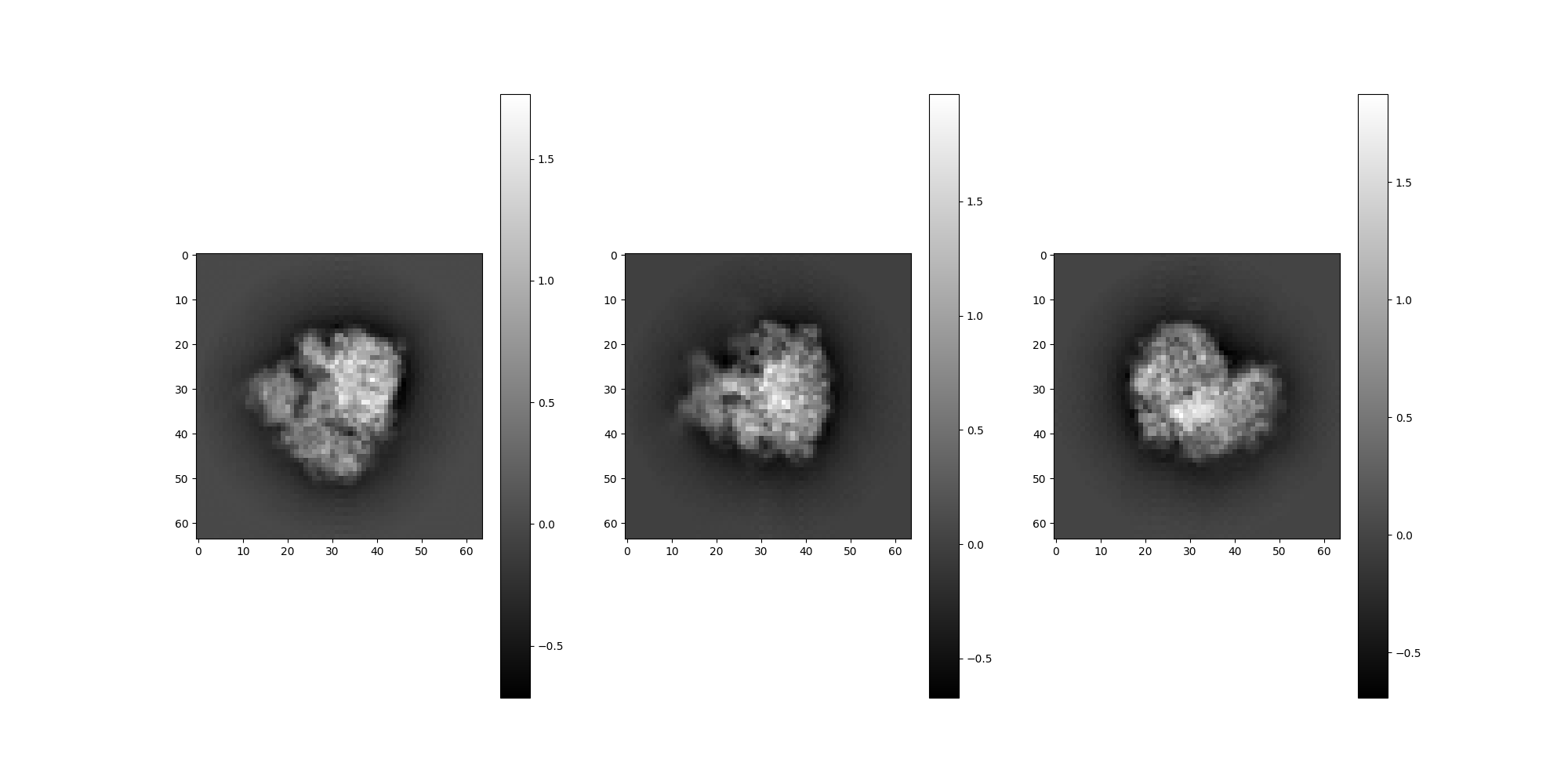
Plot Data

For quick sanity checking purposes we can view some plots.

We’ll use three orthographic projections, one per axis.

orthographic_projections = np.empty((3, L, L), dtype=vol_ds.dtype)
for i in range(3):
    orthographic_projections[i] = np.sum(vol_ds, axis=(0, i + 1))
Image(orthographic_projections).show()

Rotation Class

While you may bring your own 3x3 matrices or generate manually (say from your own Euler angles), ASPIRE has a Rotation class which can do this random rotation generation for us. It also has some other utility methods, including support for Rodrigues rotations (ie, axis-angle). Other ASPIRE components dealing with 3D rotations will generally expect instances of Rotation.

A common task in computational cryo-EM is generating random projections, by applying random 3D rotations to a volume and projecting along the z-axis. The following code will generate some random rotations, and use the Volume.project() method to return an Image instance representing the stack of projections. We can display projection images using the Image.show() method.

from aspire.utils import Rotation

num_rotations = 2
rots = Rotation.generate_random_rotations(n=num_rotations, seed=12345)

We can access the Numpy array holding the actual stack of 3x3 matrices:

print(rots)
print(rots.matrices)

Rotation stack consisting of 2 elements of float32 type
[[[ 0.34373102 -0.62564886  0.7002946 ]
  [-0.61950386 -0.7115173  -0.33159938]
  [ 0.70573646 -0.3198542  -0.63216245]]

 [[ 0.3189953   0.88963485 -0.3267902 ]
  [ 0.67460066  0.02905637  0.7376108 ]
  [ 0.6656996  -0.45574725 -0.5908794 ]]]

Using the Volume.project() method we compute projections using the stack of rotations:

projections = vol.project(rots)
print(projections)

2 float32 images arranged as a (2,) stack each of size 360x360.

project() returns an Image instance, so we can call show.

projections.show()

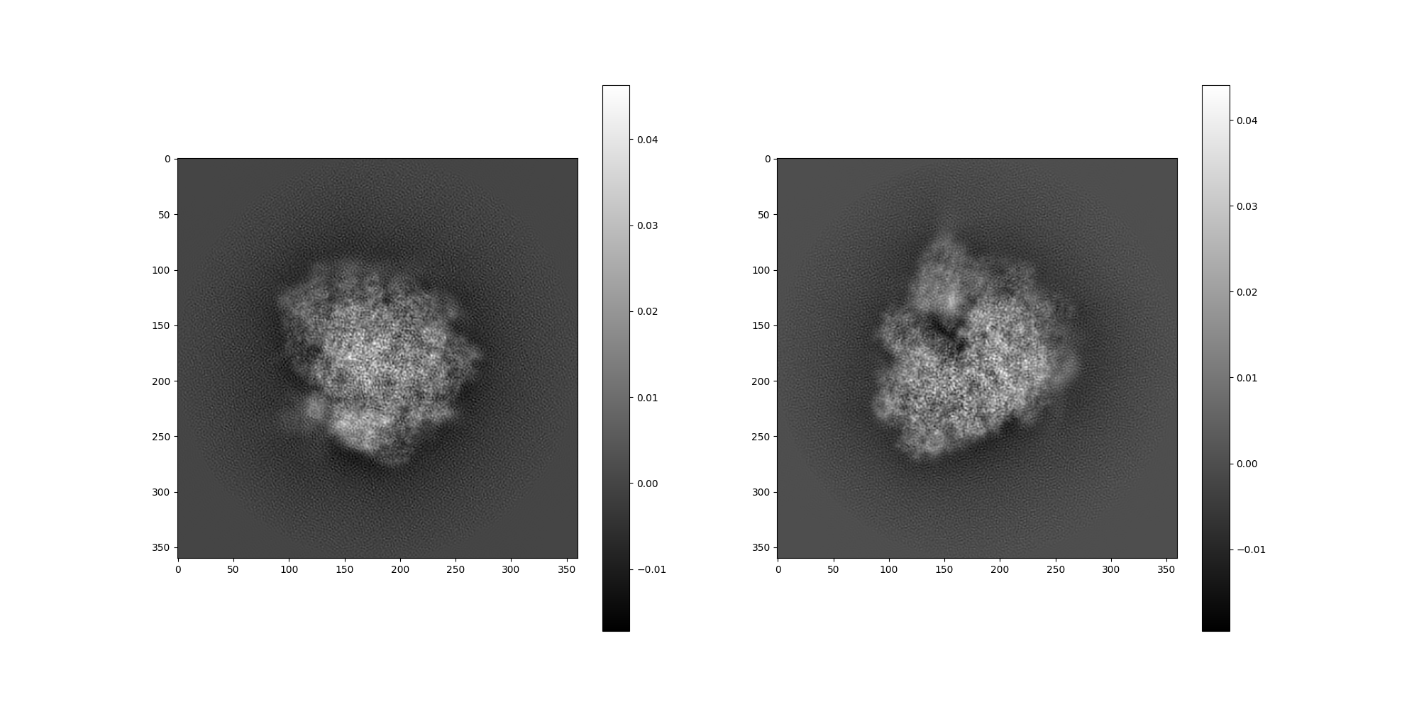
Neat, we’ve generated random projections of some real data. This tutorial will go on to show how this can be performed systematically with other cryo-EM data simulation tasks.

The filter Package

Filters are a collection of classes which once configured can be applied to Images, typically in an ImageSource pipeline which will be discussed in a later section. Specifically, applying a Filter convolves the filter with the images contained in the Image instance.

classDiagram class Filter{ +evaluate() +basis_mat() +scale() +evaluate_grid() +dual() +sign() } Filter o-- FunctionFilter Filter o-- ArrayFilter Filter o-- ScalarFilter Filter o-- ZeroFilter Filter o-- IdentityFilter Filter o-- CTFFilter CTFFilter o-- RadialCTFFilter

CTFFilter and RadialCTFFilter are the most common filters encountered when starting out and are detailed in CTF: Contrast Transfer Function. The other filters are used behind the scenes in components like NoiseAdders or more advanced customized pipelines. Several filters for internal or advanced use cases are omitted from the diagram, but can be found in the aspire.operators.filter module.

Basis

ASPIRE provides a selection of Basis classes designed for working with cryo-EM data in two and three dimensions. Most of these basis implementations are optimized for efficient rotations, often called the “steerable” property. As of this writing most algorithms in ASPIRE are written to work well with the fast Fourier-Bessel (FFB) basis classes FFBBasis2D and FFBBasis3D. These correspond to direct slower reference FBBasis2D and FBBasis3D classes.

Recently, a related Fourier-Bessel method using fast Laplacian eigenfunction (FLE) transforms was integrated as FLEBasis2D. Additional prolate spheroidal wave function (PSWF) methods are available via FPSWFBasis2D and FPSWFBasis3D, but their integration into other components like 2D covariance analysis is incomplete, and slated for a future release.

The source Package

The aspire.source package contains a collection of data source interfaces. Ostensibly, a Source is a producer of some primitive type, most notably Image. ASPIRE components that consume (process) images are designed to accept an ImageSource.

The first reason for this is to normalize the way a wide variety of higher-level components interface. ImageSource instances have a consistent property images which must be implemented to serve up images dynamically using a square-bracket [] syntax familiar to Numpy users. This supports batch computation among other things. Source instances also store and serve up metadata like rotations, dtype, and support pipelining transformations.

The second reason is so we can design an experiment using a synthetic Simulation source or our own provided Numpy arrays via ArrayImageSource and then later swap out the source for a large experimental data set using something like RelionSource. Experimental datasets can be too large to practically fit or process entirely in memory, and force the use of iteratively-batched approaches.

Generally, the source package attempts to make most of this opaque to an end user. Ideally we can simply swap one source for another. For now we will build up to the creation and application of synthetic data set based on the various manual interactions above.

classDiagram class ImageSource{ +L +n +dtype ... +images[] +cache() +downsample() +whiten() +phase_flip() +invert_conrast() +normalize_background() +save() +save_images() ... } ImageSource o-- ArrayImageSource ImageSource o-- Simulation ImageSource o-- RelionSource ImageSource o-- CoordinateSource CoordinateSource o-- BoxesCoordinateSource CoordinateSource o-- CentersCoordinateSource

Simulation Class

Generating realistic synthetic data sources is a common task. The process of generating then projecting random rotations is integrated into the Simulation class. Using Simulation, we can generate arbitrary numbers of projections for use in experiments. Then additional features are introduced which allow us to create more realistic data sources.

from aspire.source import Simulation

# Total images in our source.
num_imgs = 100

Generate a Simulation instance based on the original volume data.

sim = Simulation(n=num_imgs, vols=vol)
# Display the first 10 images
sim.images[:10].show()  # Hi Res

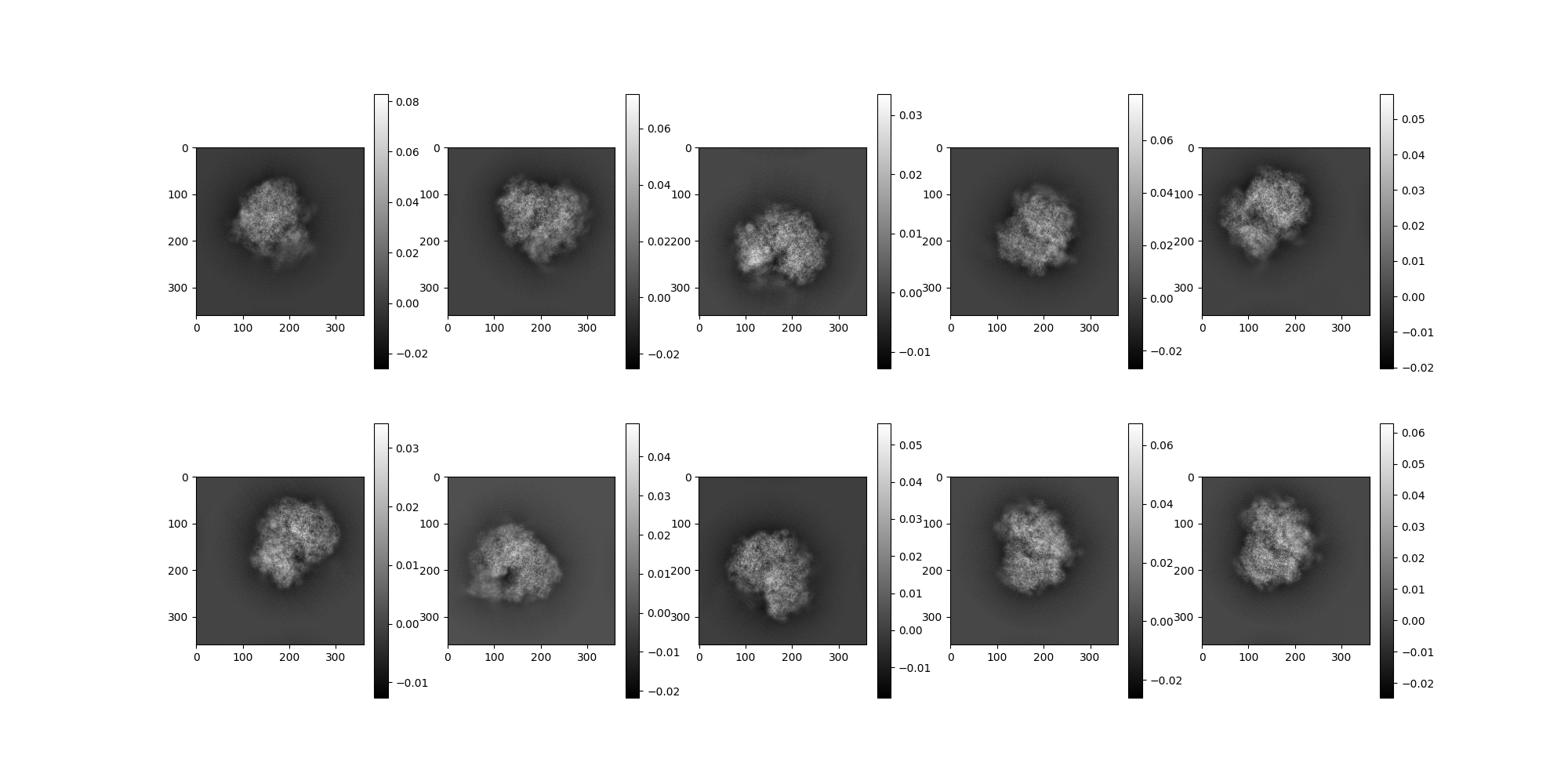
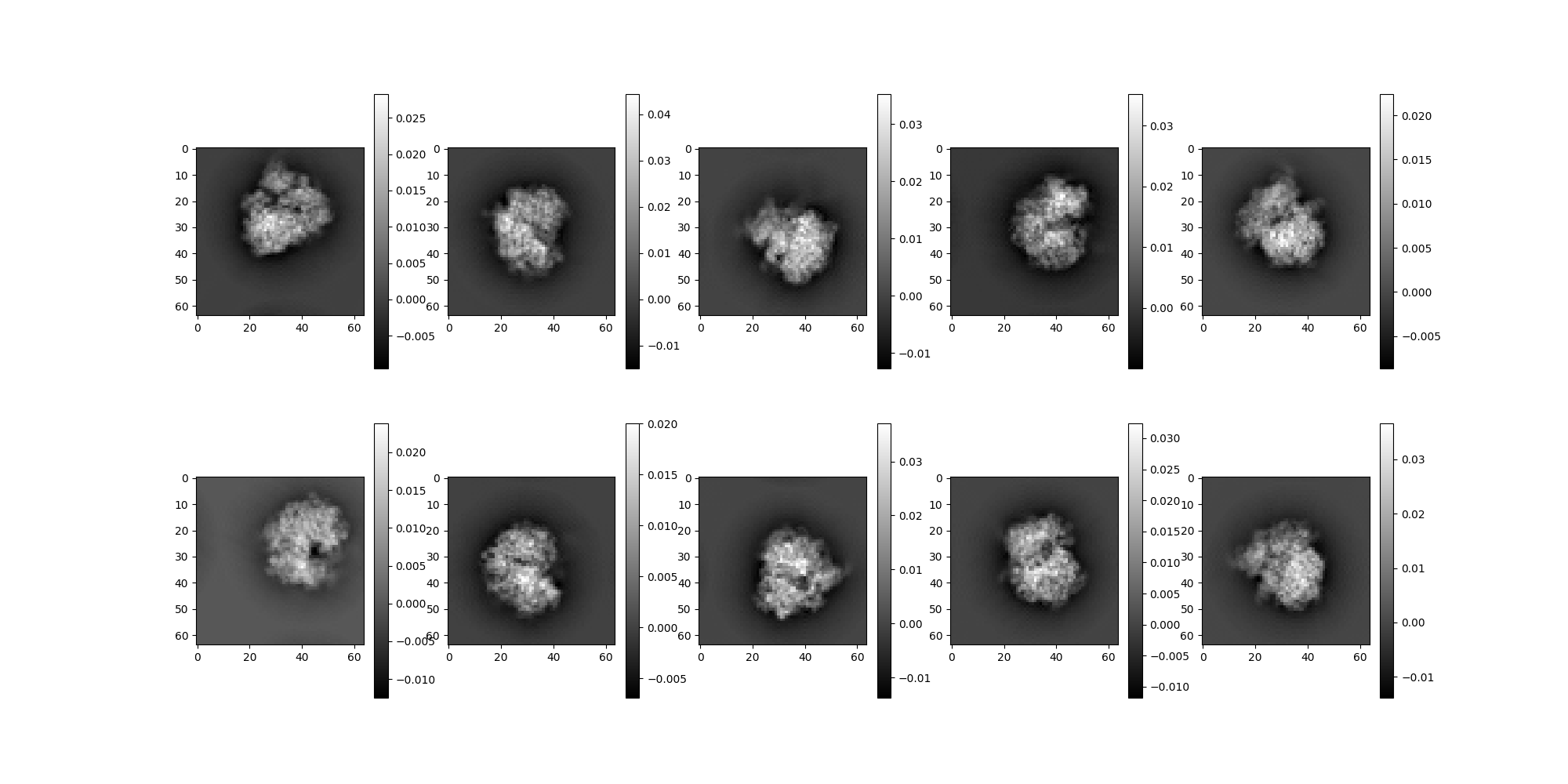
Repeat for the lower resolution (downsampled) volume vol_ds.

sim = Simulation(n=num_imgs, vols=vol_ds)
sim.images[:10].show()  # Lo Res

Note both of those simulations have the same rotations because they had the same seed by default, We recreate sim with a distinct seed to get different random samples (of rotations).

sim = Simulation(n=num_imgs, vols=vol_ds, seed=42)
sim.images[:10].show()

We can also view the rotations used to create these projections.

print(sim.rotations)

[[[ 0.1374932   0.9594606  -0.24603027]
  [ 0.9659938  -0.07497529  0.24745627]
  [ 0.21897836 -0.27168727 -0.93714166]]

 [[ 0.37807834  0.132081    0.9163031 ]
  [ 0.40860063  0.8643426  -0.29318497]
  [-0.83072394  0.48524892  0.27282083]]

 [[ 0.86643094  0.48816934 -0.10482421]
  [ 0.09854265 -0.37300435 -0.92258173]
  [-0.48947603  0.7890237  -0.37128803]]

 [[-0.35693905  0.45857018 -0.81382304]
  [ 0.47638273 -0.6600464  -0.58085996]
  [-0.803526   -0.5950228   0.01714141]]

 [[ 0.15889233  0.93312883  0.32252717]
  [-0.87645537 -0.01707341  0.48118034]
  [ 0.45450988 -0.35913652  0.8151329 ]]

 [[-0.32674402 -0.8130629   0.48183718]
  [-0.38360518  0.58002734  0.7186204 ]
  [-0.8637624   0.04996968 -0.5014156 ]]

 [[-0.34698084 -0.1871273   0.9190145 ]
  [ 0.5046363   0.78870445  0.35112315]
  [-0.79053557  0.5856011  -0.1792341 ]]

 [[-0.8140751  -0.09364705  0.57315964]
  [-0.37379512 -0.6708314  -0.64051735]
  [ 0.44447604 -0.7356735   0.5111023 ]]

 [[ 0.45521852  0.5792567  -0.6761936 ]
  [ 0.29612732 -0.81470734 -0.49855846]
  [-0.8396932   0.02671366 -0.54240364]]

 [[ 0.93491715  0.32658473 -0.13882485]
  [ 0.21361442 -0.83031636 -0.5147267 ]
  [-0.28337044  0.45157185 -0.84604025]]

 [[ 0.43646738 -0.00271971  0.89971596]
  [-0.24721187 -0.9618694   0.11701906]
  [ 0.865091   -0.27349547 -0.420497  ]]

 [[ 0.06204434 -0.68872344  0.7223645 ]
  [-0.9629127  -0.23171897 -0.13822247]
  [ 0.26258263 -0.686998   -0.6775574 ]]

 [[-0.9549782  -0.15465972  0.2531738 ]
  [ 0.02725631 -0.8954967  -0.44423273]
  [ 0.2954212  -0.417332    0.8593953 ]]

 [[-0.9362025  -0.29906207  0.1846258 ]
  [ 0.32780164 -0.553521    0.7656113 ]
  [-0.12677105  0.77728784  0.6162408 ]]

 [[ 0.8579973   0.321847    0.40031877]
  [-0.46083617  0.13809928  0.8766748 ]
  [ 0.2268714  -0.93666595  0.26680756]]

 [[-0.88663757 -0.37402767  0.27198744]
  [ 0.45935175 -0.64413124  0.6116297 ]
  [-0.05357084  0.6672318   0.7429212 ]]

 [[-0.74606377  0.6106348  -0.26554468]
  [-0.55859023 -0.35687232  0.748745  ]
  [ 0.36244422  0.7069422   0.60734415]]

 [[-0.16853625  0.61572605 -0.7697252 ]
  [ 0.9855458   0.11886839 -0.12070518]
  [ 0.01717467 -0.7789427  -0.6268599 ]]

 [[ 0.7561905  -0.33249253 -0.563582  ]
  [ 0.5429612   0.79951745  0.2568366 ]
  [ 0.3651974  -0.50022054  0.785118  ]]

 [[ 0.77301854 -0.58071446 -0.25536844]
  [ 0.25237784 -0.08780504  0.9636367 ]
  [-0.5820204  -0.8093584   0.07868452]]

 [[-0.28316504 -0.7468036  -0.6017491 ]
  [ 0.8560133   0.08614567 -0.5097256 ]
  [ 0.43250299 -0.6594417   0.6148803 ]]

 [[-0.14112386  0.9097205   0.3905032 ]
  [-0.8198382  -0.3284985   0.46899253]
  [ 0.5549318  -0.2539634   0.7921826 ]]

 [[-0.456592   -0.85562974 -0.2437653 ]
  [-0.4374926  -0.02264298  0.89893687]
  [-0.7746767   0.5170929  -0.36399308]]

 [[-0.90090746  0.11707234 -0.4179232 ]
  [-0.10193092  0.8789243   0.4659422 ]
  [ 0.4218718   0.4623701  -0.7798962 ]]

 [[-0.3212181  -0.4951543  -0.80724293]
  [-0.94361854  0.2393791   0.22865206]
  [ 0.08001903  0.8351765  -0.54412967]]

 [[ 0.97377276  0.06877314  0.21687981]
  [ 0.22443582 -0.13386007 -0.96525127]
  [-0.03735181  0.98861104 -0.14578445]]

 [[ 0.3553472  -0.9034085   0.23996124]
  [ 0.5433438   0.4085248   0.7334064 ]
  [-0.76059574 -0.13023247  0.63602954]]

 [[ 0.61806667  0.37726    -0.68968725]
  [-0.56937826  0.8197457  -0.06184895]
  [ 0.54203504  0.4309197   0.7214612 ]]

 [[ 0.29776493  0.94447404 -0.13894197]
  [ 0.9458294  -0.31160298 -0.09116108]
  [-0.129394   -0.10427082 -0.9860957 ]]

 [[ 0.19716634  0.21056637  0.9574901 ]
  [-0.7070152  -0.64604855  0.2876643 ]
  [ 0.6791575  -0.73367774  0.0214946 ]]

 [[-0.5650243   0.2975922  -0.7695365 ]
  [ 0.7782365  -0.11755076 -0.616871  ]
  [-0.27403557 -0.94742846 -0.16517805]]

 [[ 0.28065482  0.8733582   0.39809337]
  [ 0.47991556 -0.4868837   0.72981185]
  [ 0.83121234 -0.013774   -0.55578446]]

 [[ 0.8024307   0.02780645  0.5960972 ]
  [-0.1587728  -0.9529598   0.25818375]
  [ 0.5752358  -0.30181855 -0.7602692 ]]

 [[ 0.32265848 -0.30083787  0.8974342 ]
  [-0.05781392 -0.9526389  -0.29855752]
  [ 0.94474816  0.04444793 -0.32476965]]

 [[ 0.4935579  -0.7422682   0.4532532 ]
  [ 0.85551316  0.5081454  -0.09942588]
  [-0.15651786  0.4368365   0.8858194 ]]

 [[-0.8976416  -0.2857157   0.33556828]
  [-0.41022733  0.26334086 -0.8731352 ]
  [ 0.1610996  -0.92142177 -0.35359412]]

 [[-0.9217232   0.19335265 -0.3362159 ]
  [-0.33698434  0.02991741  0.9410348 ]
  [ 0.19201028  0.9806731   0.03758125]]

 [[ 0.24043691 -0.61969984  0.74710256]
  [ 0.35552713  0.7724179   0.5262804 ]
  [-0.90321124  0.13907799  0.40603787]]

 [[-0.79218084 -0.47242948 -0.38634163]
  [ 0.16552027  0.4430016  -0.88110876]
  [ 0.5874117  -0.76194483 -0.27274075]]

 [[-0.71742296  0.624828   -0.30804914]
  [-0.68107444 -0.7220424   0.12162399]
  [-0.14643046  0.29706025  0.9435642 ]]

 [[ 0.87354153 -0.40243074  0.27381516]
  [ 0.33415928  0.9048438   0.26380917]
  [-0.35392484 -0.13895038  0.9248946 ]]

 [[ 0.48421115  0.11260304 -0.8676751 ]
  [ 0.27090228 -0.96224743  0.02630238]
  [-0.83195645 -0.24779108 -0.49643534]]

 [[ 0.10466753 -0.18718329  0.9767329 ]
  [-0.49893624  0.83970237  0.21438888]
  [-0.86029494 -0.509767   -0.00550296]]

 [[ 0.62265253 -0.1254365   0.7723791 ]
  [ 0.46602726 -0.7334752  -0.49480575]
  [ 0.6285876   0.66804177 -0.39824337]]

 [[-0.07320143 -0.99607444 -0.04977208]
  [-0.4329861  -0.01321644  0.9013037 ]
  [-0.8984234   0.08752733 -0.43031895]]

 [[ 0.06439321  0.97830254 -0.19692044]
  [ 0.938444   -0.12647285 -0.32144594]
  [-0.33937648 -0.16409987 -0.92622614]]

 [[-0.32914323  0.8692355  -0.36890975]
  [-0.34743685  0.2517924   0.9032653 ]
  [ 0.87803894  0.4254765   0.21912868]]

 [[-0.03135481  0.12190165 -0.99204683]
  [ 0.20567426 -0.9705069  -0.12575543]
  [-0.97811806 -0.20798153  0.00535803]]

 [[ 0.7707965   0.4763445  -0.42304692]
  [ 0.4696665  -0.8735372  -0.12785189]
  [-0.43044877 -0.10014319 -0.89704245]]

 [[ 0.62561727 -0.6937239   0.3568615 ]
  [-0.5623879  -0.08402125  0.8225936 ]
  [-0.54066896 -0.7153234  -0.44270706]]

 [[-0.0384063  -0.82296616  0.5667907 ]
  [ 0.98650855 -0.12155963 -0.10965481]
  [ 0.15914106  0.5549324   0.8165318 ]]

 [[ 0.71410507 -0.68704677  0.13424107]
  [-0.28213766 -0.45796394 -0.8430109 ]
  [ 0.6406655   0.5641239  -0.52087617]]

 [[-0.6900714  -0.31053716  0.65373397]
  [-0.5909326   0.76325965 -0.26121518]
  [-0.41785175 -0.56656986 -0.7102102 ]]

 [[ 0.56709814 -0.23533636  0.7893139 ]
  [ 0.71543354 -0.3340903  -0.6136274 ]
  [ 0.40811095  0.9126886  -0.02109447]]

 [[ 0.12042121  0.97353137 -0.1942559 ]
  [-0.98601013  0.09457708 -0.13725594]
  [-0.1152508   0.20806682  0.9713009 ]]

 [[ 0.26161245 -0.60064805  0.75550044]
  [-0.5359779  -0.74138415 -0.40382826]
  [ 0.80267465 -0.29928502 -0.51588935]]

 [[ 0.4752947  -0.37172344  0.7974438 ]
  [-0.1643763   0.852889    0.4955409 ]
  [-0.86433524 -0.36660883  0.3442711 ]]

 [[ 0.83131063  0.47794443  0.28371063]
  [-0.4780851   0.35454985  0.80357265]
  [ 0.28347355 -0.80365634  0.5232392 ]]

 [[ 0.5751311   0.03900156  0.817131  ]
  [-0.27594915 -0.93107     0.23866446]
  [ 0.7701144  -0.36274996 -0.5247249 ]]

 [[-0.6807762  -0.6099538  -0.4055862 ]
  [ 0.07149926 -0.6063983   0.79194   ]
  [-0.7289936   0.51013476  0.45643273]]

 [[ 0.27400538  0.6167242  -0.73795146]
  [ 0.63375145  0.46136382  0.6208885 ]
  [ 0.72338104 -0.63780457 -0.2644337 ]]

 [[ 0.02657236 -0.9912923  -0.12897094]
  [ 0.27007505 -0.11709963  0.955692  ]
  [-0.96247256 -0.06022682  0.2646117 ]]

 [[ 0.75919664  0.46289822  0.4575431 ]
  [ 0.21626568  0.4836275  -0.84813535]
  [-0.61388075  0.7428524   0.2670594 ]]

 [[ 0.13419726  0.7730551  -0.6199814 ]
  [ 0.01575051  0.62389755  0.7813474 ]
  [ 0.99082947 -0.11461972  0.07154934]]

 [[ 0.7969387  -0.5938283  -0.11070973]
  [-0.44239753 -0.6985636   0.5623996 ]
  [-0.41130662 -0.39922032 -0.8194205 ]]

 [[-0.2271311  -0.6608967  -0.71528107]
  [ 0.9729143  -0.12155605 -0.19662634]
  [ 0.04300295 -0.74056715  0.670605  ]]

 [[ 0.8058346   0.03859079  0.5908818 ]
  [-0.50750047 -0.4691095   0.7227583 ]
  [ 0.3050801  -0.88229644 -0.35843983]]

 [[-0.84541976 -0.47147918  0.25094387]
  [-0.48244947  0.47254407 -0.737526  ]
  [ 0.22914612 -0.74458677 -0.62696296]]

 [[ 0.17157505  0.919783    0.35293233]
  [ 0.95262057 -0.24622187  0.17857464]
  [ 0.25114956  0.30557165 -0.9184497 ]]

 [[ 0.03022777 -0.19667654  0.98000234]
  [ 0.96350527 -0.25516328 -0.0809276 ]
  [ 0.26597717  0.9466837   0.18178587]]

 [[-0.9041375   0.4069089   0.1302327 ]
  [-0.2578785  -0.276723   -0.9257014 ]
  [-0.34063777 -0.8705455   0.3551287 ]]

 [[ 0.76876014 -0.6344005   0.0808938 ]
  [-0.632561   -0.7356355   0.24229503]
  [-0.09420373 -0.23743702 -0.96682435]]

 [[ 0.04193976 -0.00535577  0.9991058 ]
  [-0.7404277   0.6712408   0.03467938]
  [-0.6708263  -0.74122     0.02418612]]

 [[-0.6622805   0.6703488   0.33468935]
  [ 0.2214073   0.6018422  -0.7673101 ]
  [-0.7157956  -0.43407184 -0.5470085 ]]

 [[ 0.00894121 -0.96657425 -0.2562309 ]
  [ 0.2980998   0.24716657 -0.92197895]
  [ 0.9544928  -0.06813876  0.29034555]]

 [[-0.09509465 -0.9904526  -0.09980346]
  [-0.64432764  0.13766429 -0.75225693]
  [ 0.75881416 -0.00722948 -0.6512671 ]]

 [[-0.93059725  0.34470695  0.12314969]
  [-0.2402517  -0.32136244 -0.91597235]
  [-0.27616635 -0.8819883   0.38187546]]

 [[ 0.48192862  0.10002194  0.87048286]
  [-0.66315746 -0.60768265  0.43697143]
  [ 0.57268405 -0.7878562  -0.22652936]]

 [[ 0.90507764 -0.29453734 -0.30672824]
  [ 0.39986134  0.83494043  0.37813416]
  [ 0.14472517 -0.46488953  0.87346   ]]

 [[ 0.48447588 -0.70774704  0.51417625]
  [-0.8526892  -0.25072426  0.4583214 ]
  [-0.19545916 -0.66047823 -0.7249581 ]]

 [[-0.64288104  0.45185107  0.6184938 ]
  [-0.23015156  0.6562045  -0.71862775]
  [-0.73057115 -0.6043395  -0.31786725]]

 [[ 0.30517054 -0.8374807  -0.4533178 ]
  [-0.89213204 -0.0849021  -0.44372523]
  [ 0.33312368  0.53983116 -0.773053  ]]

 [[-0.32206497  0.9112062  -0.25686076]
  [-0.869473   -0.17734958  0.46104652]
  [ 0.37455428  0.37182042  0.8493872 ]]

 [[ 0.3610673  -0.7101037   0.6044693 ]
  [ 0.7567135   0.60192007  0.2551017 ]
  [-0.5449909   0.36530122  0.7546787 ]]

 [[ 0.27847555  0.90301734 -0.3271255 ]
  [ 0.5723424   0.11749125  0.811554  ]
  [ 0.7712817  -0.41322574 -0.48411667]]

 [[-0.3412885  -0.83527166 -0.43109557]
  [ 0.17580529 -0.50726277  0.84366876]
  [-0.9233714   0.21214558  0.3199681 ]]

 [[ 0.2919039  -0.9513335  -0.09877586]
  [ 0.5871929   0.25977072 -0.76663136]
  [ 0.75498116  0.16578221  0.63444436]]

 [[-0.1322668  -0.75247324 -0.645205  ]
  [ 0.2528478   0.60377645 -0.75599074]
  [ 0.9584224  -0.26313114  0.11040162]]

 [[ 0.62349445 -0.19195779  0.75789636]
  [ 0.7480926  -0.13520728 -0.6496741 ]
  [ 0.2271831   0.9720449   0.05930121]]

 [[-0.33402812  0.42084855 -0.84339297]
  [ 0.6074924   0.7802727   0.14875284]
  [ 0.720679   -0.4626672  -0.5162954 ]]

 [[-0.7137928  -0.55692726  0.424655  ]
  [-0.4062189   0.8231522   0.39674512]
  [-0.57051384  0.11069094 -0.8137945 ]]

 [[ 0.04948919  0.98905236 -0.13901873]
  [-0.8053667  -0.04280363 -0.59122956]
  [-0.5907075   0.14122052  0.7944315 ]]

 [[-0.87180173  0.4881775   0.04055187]
  [-0.41275278 -0.6874722  -0.597509  ]
  [-0.26381218 -0.5376473   0.8008361 ]]

 [[ 0.44658735 -0.04983776 -0.89335096]
  [-0.64957654  0.6685733  -0.3620222 ]
  [ 0.615313    0.74197435  0.26620296]]

 [[ 0.68048185  0.72213393  0.12436624]
  [ 0.31681323 -0.13690118 -0.938556  ]
  [-0.6607373   0.67807126 -0.32194036]]

 [[-0.29298428  0.08057309 -0.95271623]
  [ 0.15083717  0.98785996  0.03715903]
  [ 0.94414425 -0.132818   -0.30158085]]

 [[-0.19727235 -0.42594904 -0.8829785 ]
  [ 0.97395647 -0.18783951 -0.12698455]
  [-0.1117693  -0.8850332   0.4519114 ]]

 [[-0.58162045  0.6032319  -0.545737  ]
  [-0.80308783 -0.53260213  0.2671795 ]
  [-0.12948951  0.59367186  0.7942205 ]]

 [[-0.43661723  0.6471804   0.62491834]
  [-0.77699894 -0.621401    0.10066503]
  [ 0.45347333 -0.4416088   0.77417284]]

 [[ 0.05435671 -0.76187783  0.64543587]
  [ 0.69972587  0.49019638  0.51970303]
  [-0.71234053  0.42337883  0.5597511 ]]]

Given any Source, we can also take slices using typical slicing syntax, or provide our own iterable of indices.

sim_evens = sim[0::2]
sim_odds = sim[1::2]

# We can also generate random selections.
# Shuffle indices then take the first 5.
shuffled_inds = np.random.choice(sim.n, 5, replace=False)
sim_shuffled_subset = sim[shuffled_inds]

Underneath those slices, ASPIRE relies on IndexedSource, which we can also call direcly to remap indices.

from aspire.source import IndexedSource

sim_shuffled_subset = IndexedSource(sim, shuffled_inds)

The noise Package

The aspire.noise package contains several useful classes for generating and estimating different types of noise.

NoiseAdder

NoiseAdder subclasses are used to add common or customized noise to Simulation image generation pipelines.

WhiteNoiseAdder

WhiteNoiseAdder is the most common type of synthetic noise.

from aspire.noise import WhiteNoiseAdder

Get the sample variance, then create a NoiseAdder based on that variance.

var = np.var(sim.images[:].asnumpy())
print(f"Sample Variance: {var}")
target_noise_variance = 10.0 * var
print(f"Target Noise Variance: {target_noise_variance}")
white_noise_adder = WhiteNoiseAdder(target_noise_variance)

Sample Variance: 3.230794027331285e-05
Target Noise Variance: 0.0003230794027331285

We can customize Sources by adding stages to their generation pipeline. In this case of a Simulation source, we want to corrupt the projection images with noise. Internally the WhiteNoiseAdder creates a ScalarFilter which is multiplied (convolution) by a Gaussian random sample. Similar to before, if you require a different sample, this can be controlled via a seed.

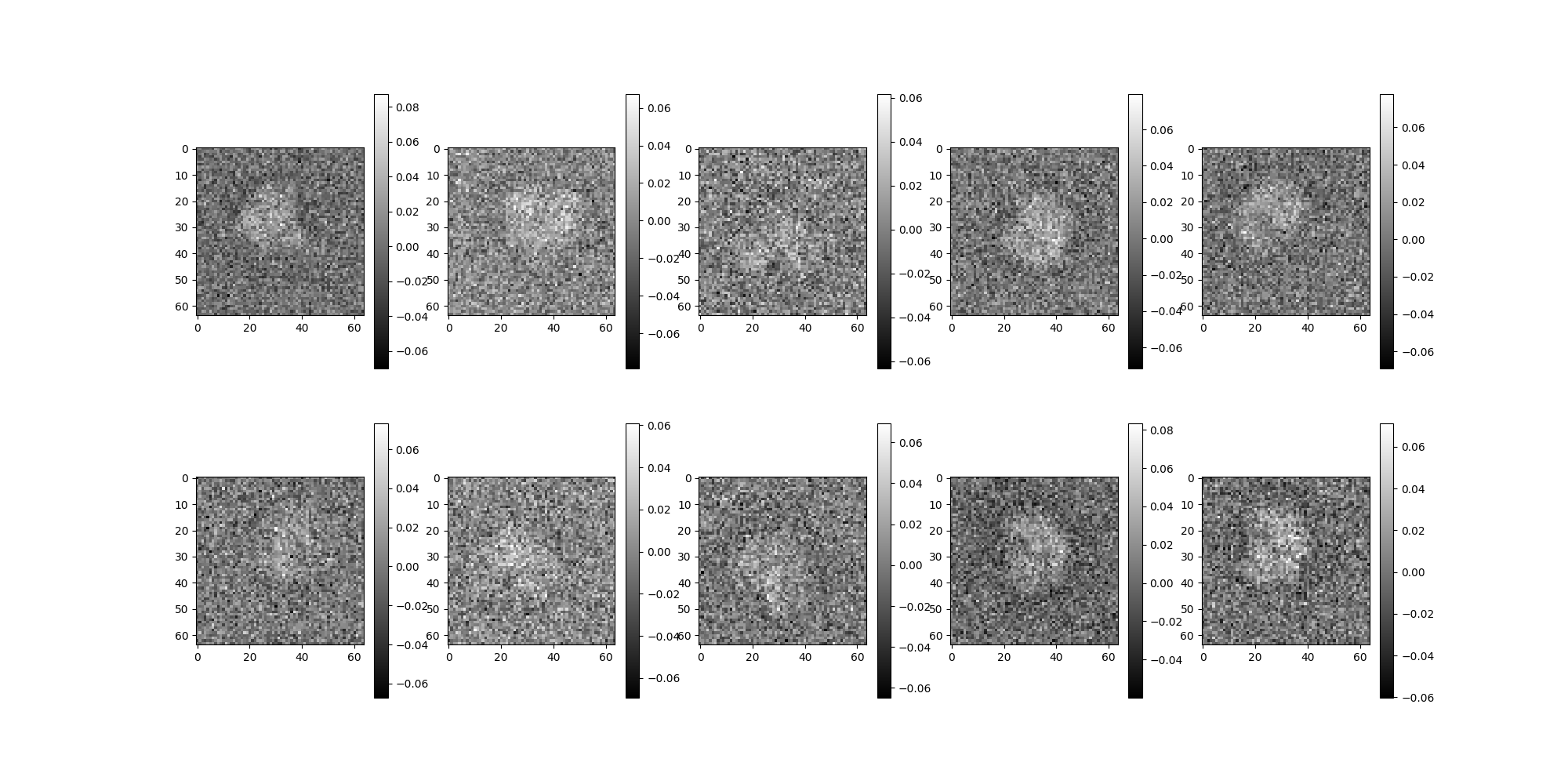
# Creating the new simulation with this additional noise is easy:
sim = Simulation(n=num_imgs, vols=vol_ds, noise_adder=white_noise_adder)
# These should be rather noisy now ...
sim.images[:10].show()

WhiteNoiseEstimator

We can estimate the noise across an ImageSource, and we’ve generated a simulation with known noise variance. Lets see how the estimate compares.

In this case, we know the noise to be white, so we can proceed directly to WhiteNoiseEstimator. The noise estimators consume from an ImageSource.

The white noise estimator should log a diagnostic variance value. Internally, it also uses the estimation results to build a Filter which can be used in more advanced denoising methods.

from aspire.noise import WhiteNoiseEstimator

noise_estimator = WhiteNoiseEstimator(sim)
noise_estimator.estimate()

  0%|          | 0/1 [00:00<?, ?it/s]
100%|██████████| 1/1 [00:00<00:00,  1.85it/s]
100%|██████████| 1/1 [00:00<00:00,  1.85it/s]

0.0003191127034369856

A Custom FunctionFilter

We will now apply some more interesting noise, using a custom function, and then apply a whitening process to our data.

Using FunctionFilter we can create our own custom functions to apply in a pipeline. Here we want to apply a custom noise function. We will use a function of two variables for this example.

from aspire.noise import CustomNoiseAdder
from aspire.operators import FunctionFilter


def noise_function(x, y):
    return 1e-7 * np.exp(-(x * x + y * y) / (2 * 0.3**2))


# In Python, functions are first class objects.  We take advantage of
# that to pass this function around as a variable.  The function is
# evaluated later, internally, during pipeline execution.
custom_noise = CustomNoiseAdder(noise_filter=FunctionFilter(noise_function))

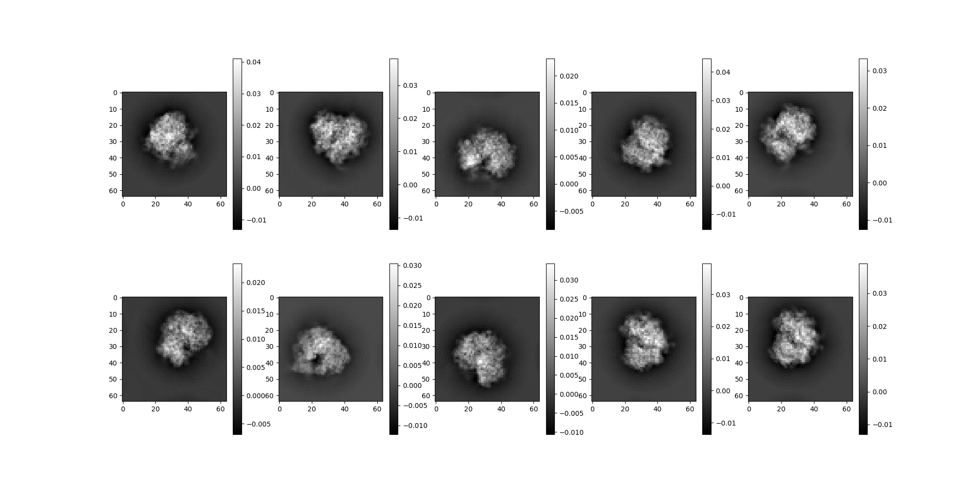
# Create yet another Simulation source to tinker with.
sim = Simulation(n=num_imgs, vols=vol_ds, noise_adder=custom_noise)
sim.images[:10].show()

Noise Whitening

We will now combine a more advanced noise estimation technique with an ImageSource preprocessing method whiten.

First an anisotropic noise estimate is performed.

from aspire.noise import AnisotropicNoiseEstimator

# Estimate noise.
aiso_noise_estimator = AnisotropicNoiseEstimator(sim)

  0%|          | 0/1 [00:00<?, ?it/s]
100%|██████████| 1/1 [00:00<00:00,  2.27it/s]
100%|██████████| 1/1 [00:00<00:00,  2.27it/s]

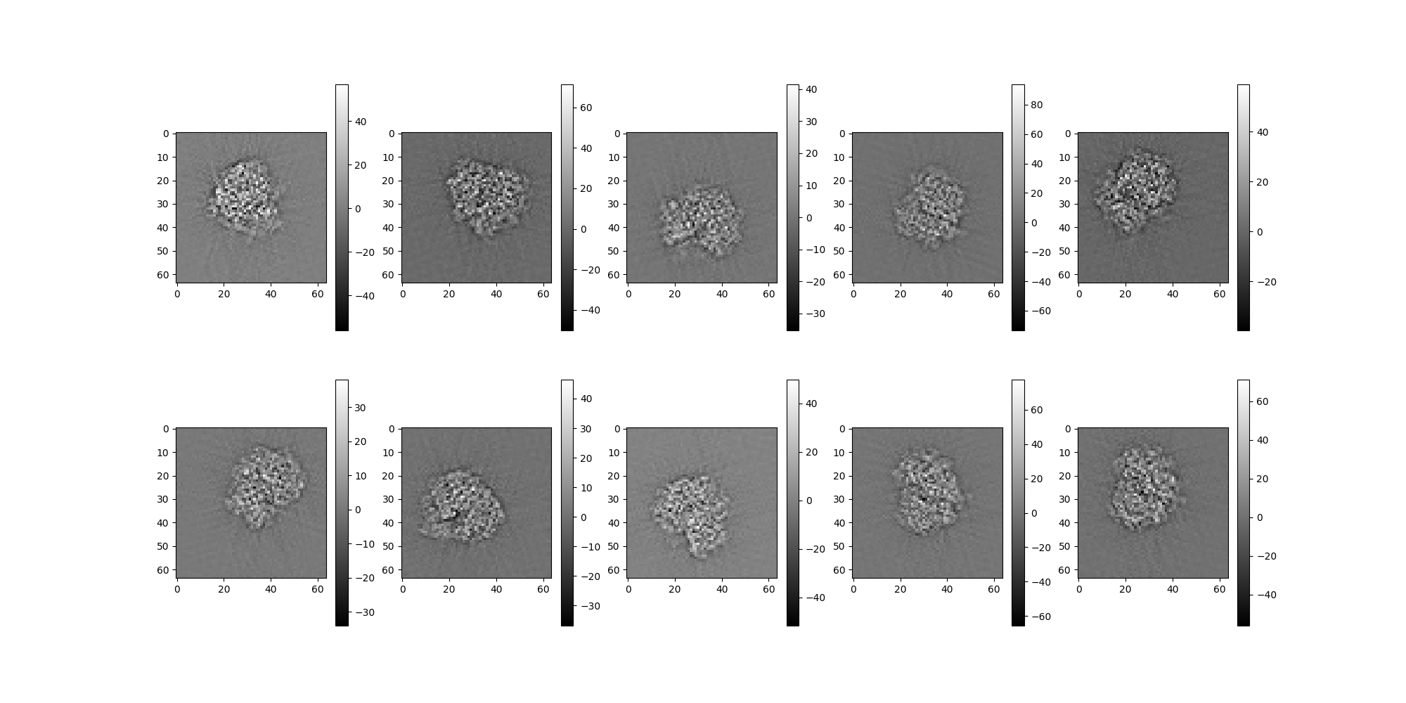
Applying the Simulation.whiten() method requires passing a corresponding NoiseEstimator instance. Then we can inspect some of the whitened images. While noise is still present, we can see a dramatic change.

# Whiten based on the estimated noise.
sim = sim.whiten(aiso_noise_estimator)

What do the whitened images look like?

sim.images[:10].show()

Common Image Corruptions

Simulation provides several configurable types of common cryo-EM image corruptions. Users should be aware that amplitude and offset corruption is enabled by default.

Amplitudes

Simulation automatically generates random amplitude variability. To disable, set to amplitudes=1.

Offsets

Simulation automatically generates random offsets. To disable, set to offsets=0.

Noise

By default, no noise corruption is configured. To enable, see NoiseAdder components.

CTF

By default, no CTF corruption is configured. To enable, we must configure one or more CTFFilter instances. Usually we will create a range of filters for a variety of defocus levels.

from aspire.operators import RadialCTFFilter

# Radial CTF Filter params.
defocus_min = 15000  # unit is angstroms
defocus_max = 25000
defocus_ct = 7

# Generate several CTFs.
ctf_filters = [
    RadialCTFFilter(pixel_size=5, defocus=d)
    for d in np.linspace(defocus_min, defocus_max, defocus_ct)
]

Combining into a Simulation

Here we’ll combine the parameters above into a new simulation.

sim = Simulation(
    n=num_imgs,
    vols=vol_ds,
    amplitudes=1,
    offsets=0,
    noise_adder=white_noise_adder,
    unique_filters=ctf_filters,
    seed=42,
)

# Simulation has two unique accessors ``clean_images`` which disables
# noise, and ``projections`` which are clean uncorrupted projections.
# Both act like calls to `image` and return show-able ``Image``
# instances.

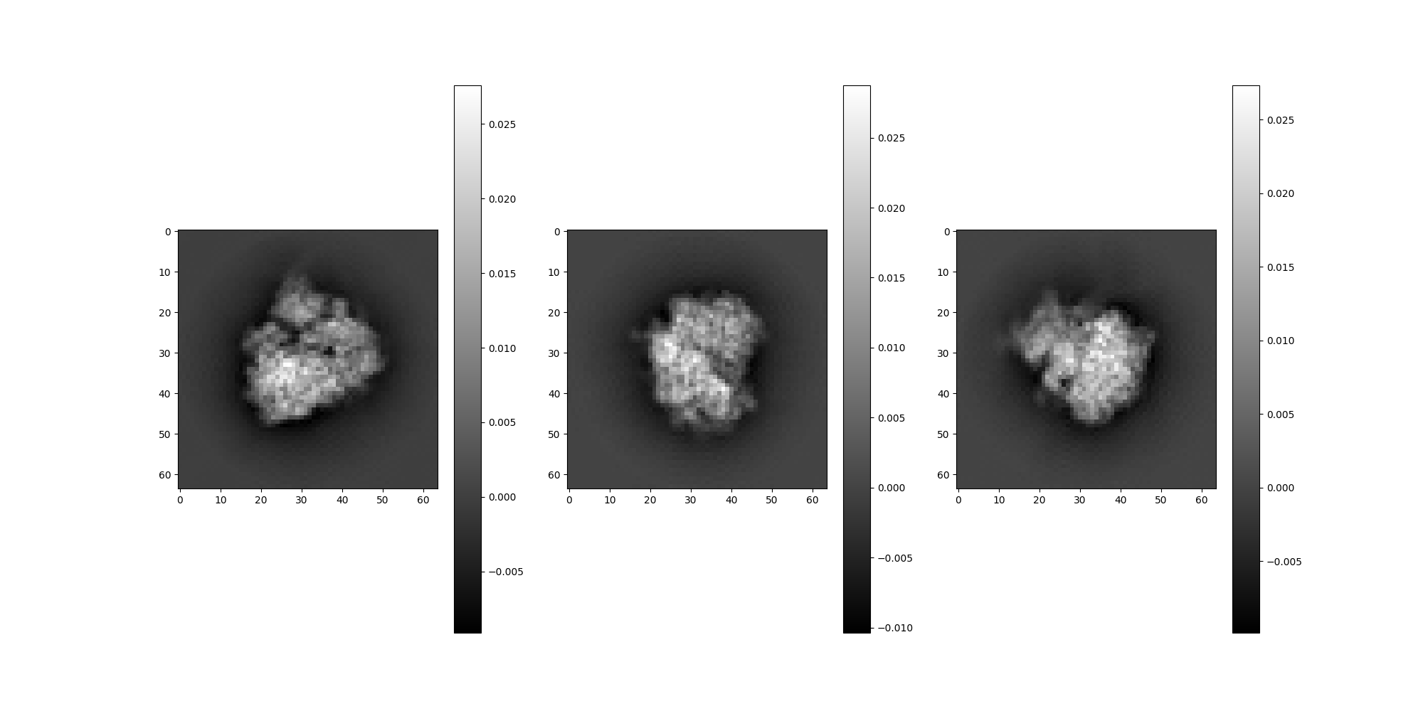
Clean projections.

sim.projections[:3].show()

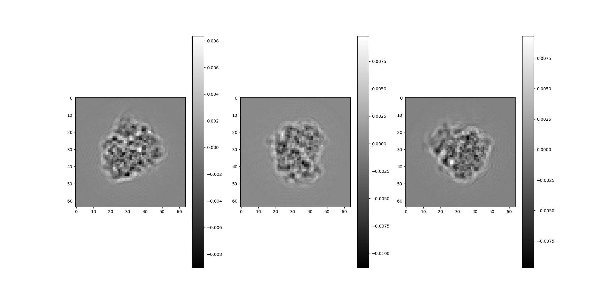
Images with only CTF applied.

sim.clean_images[:3].show()

And now the first four corrupted images.

sim.images[:4].show(columns=2, colorbar=False)

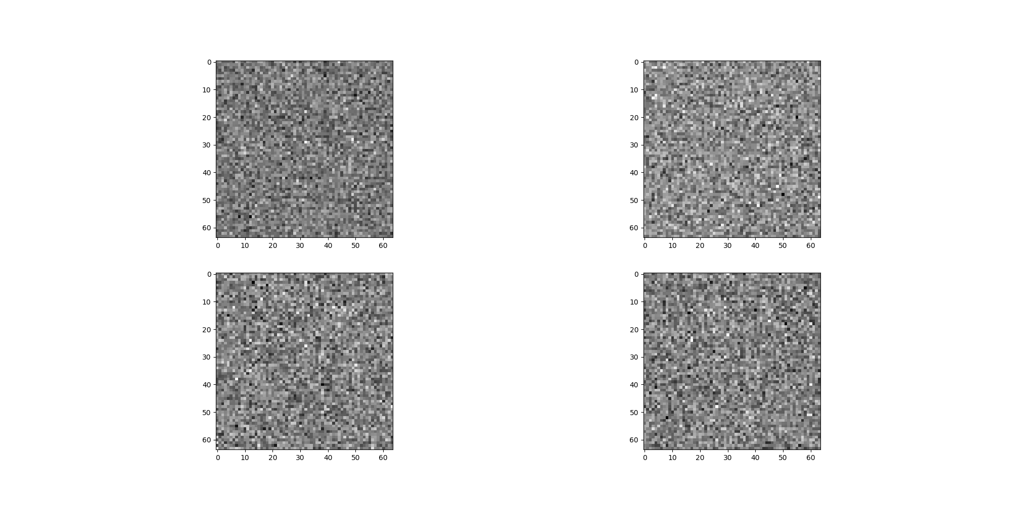
Note

Above the show call has been customized as a 2 column grid with out colorbar legend.

Real Experimental Data - RelionSource

Now that we have some basics, we can try to replace the simulation with a real experimental data source.

from aspire.source import RelionSource

src = RelionSource(
    "data/sample_relion_data.star",
    data_folder="",
    pixel_size=5.0,
    max_rows=1024,
)

Add downsampling to the src pipeline.

src = src.downsample(img_size)

RelionSource will auto-populate CTFFilter instances from the STAR file metadata when available. Having these filters allows us to perform a phase flipping correction.

src = src.phase_flip()

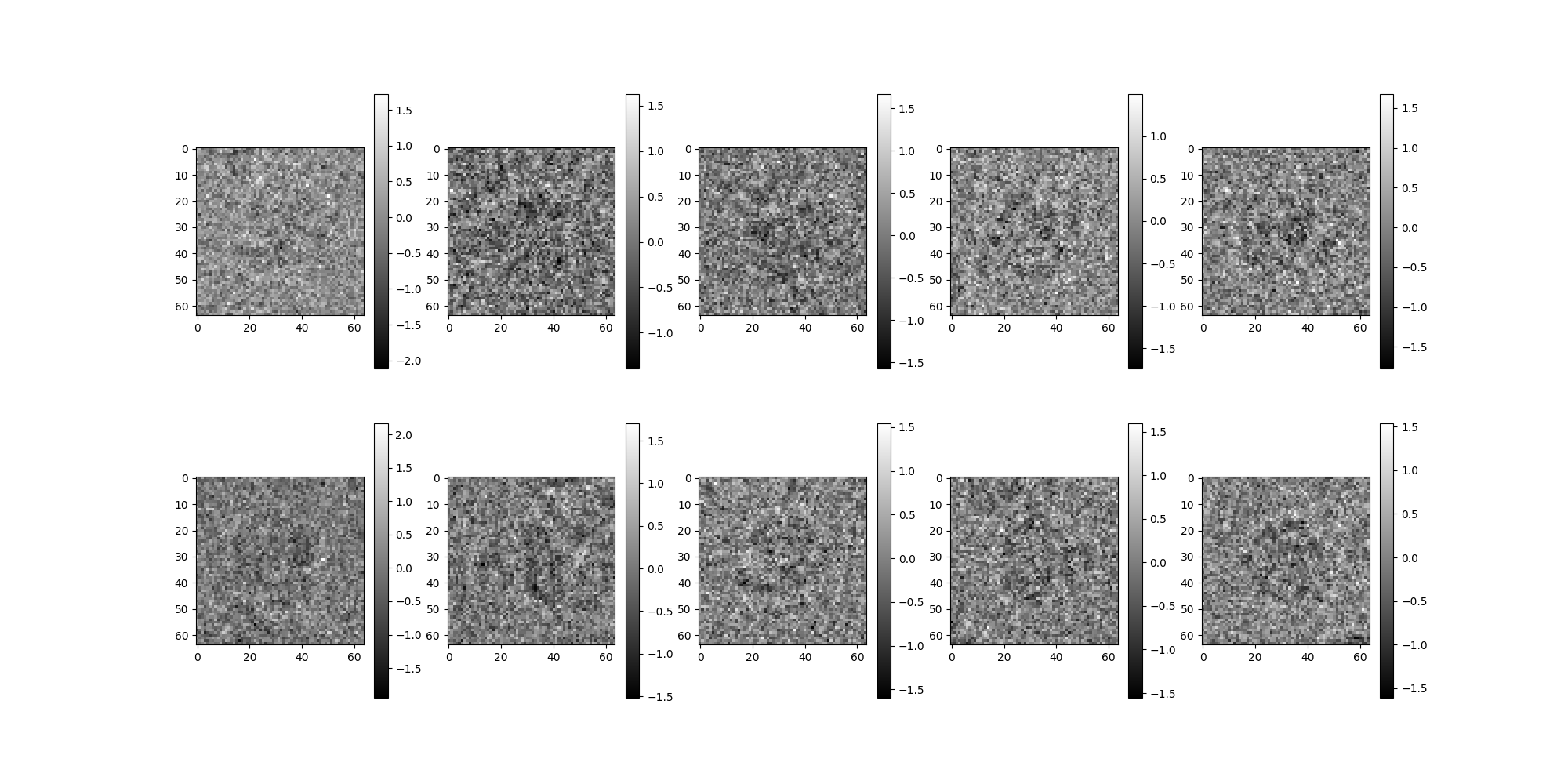
Display the experimental data images.

src.images[:10].show()

Pipeline Roadmap

Now that the primitives have been introduced we can explore higher-level components. The higher-level components are designed to be modular and cacheable (to memory or disk) to support experimentation with entire pipelines or focused algorithmic development on specific components. Most pipelines will follow a flow of data and components moving mostly left to right in the table below. This table is not exhaustive, but represents some of the most common components.

Image Processing			Ab initio
Data	Preprocessing	Denoising	Orientation	3D Reconstruction
Simulation	NoiseEstimator	Class Averaging	CLSyncVoting	MeanVolumeEstimator
RelionSource	downsample	cov2d (CWF)	CLSymmetryC2
CoordinateSource	whiten		CLSymmetryC3C4
	phase_flip		CLSymmetryCn
	normalize_background		CommonlineSDP
	CTFEstimator

We’re now ready to explore a small example end-to-end ab initio pipeline using simulated data. Ab-initio Pipeline Demonstration

Larger simulations and experiments based on EMPIAR data can be found in Experiments.